Lonely pentagons: Digging arbitrarily deep wells on a sphere


Another wild goose chase.

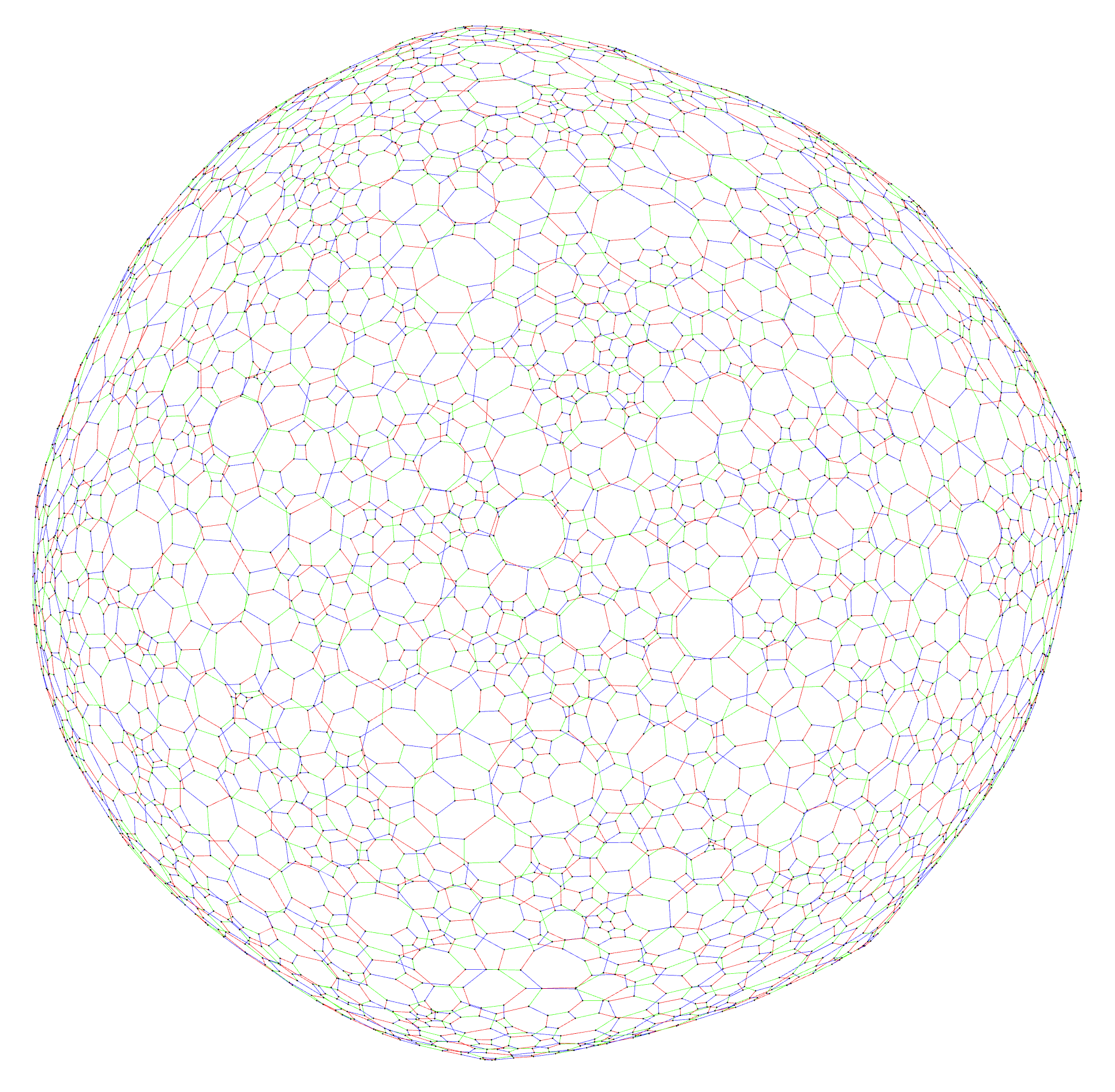
I was convinced that cubic maps on the sphere without F2, F3, and F4 faces were forced to have large clusters of F5 faces. But I’ve actually found an infinite family of counterexamples showing that it is possible to build maps of arbitrary size, with faces of arbitrary size, with no face smaller than a pentagon, and with every pentagon kept strictly isolated from every other.

Anyway, I don’t mind chasing wild geese, quite the contrary actually, because this wonderful theorem keeps showing me things I didn’t know, bringing me to the work of people I didn’t know.

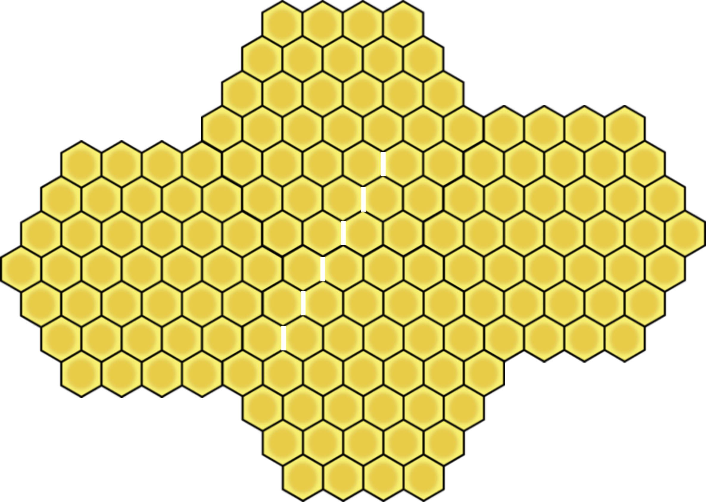
Surgery on a sea of hexagons

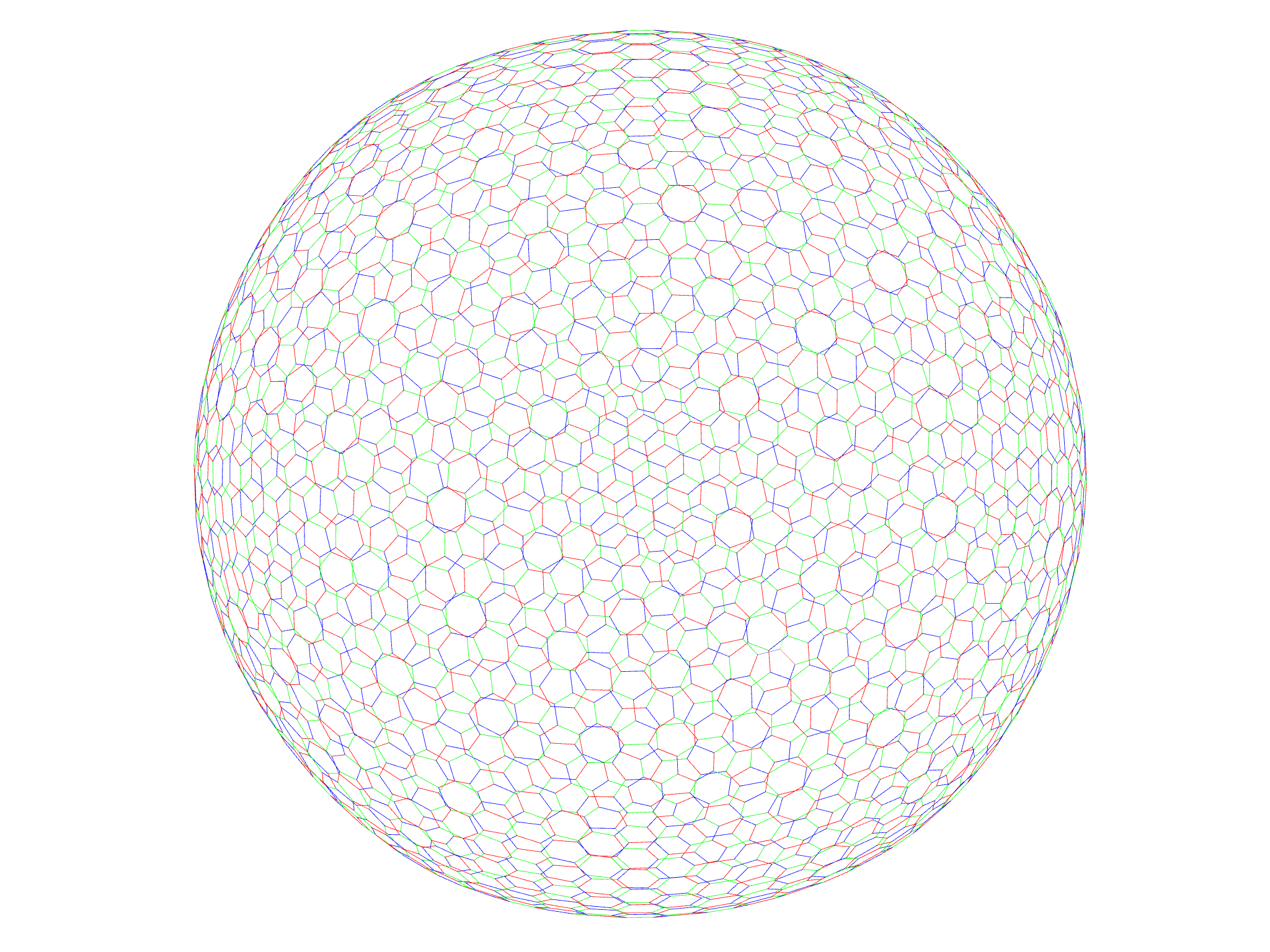
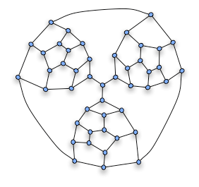
Everything below happens far out in the hexagonal ocean of a giant Goldberg map. See Fullerene structure or Goldberg polyhedron for details.

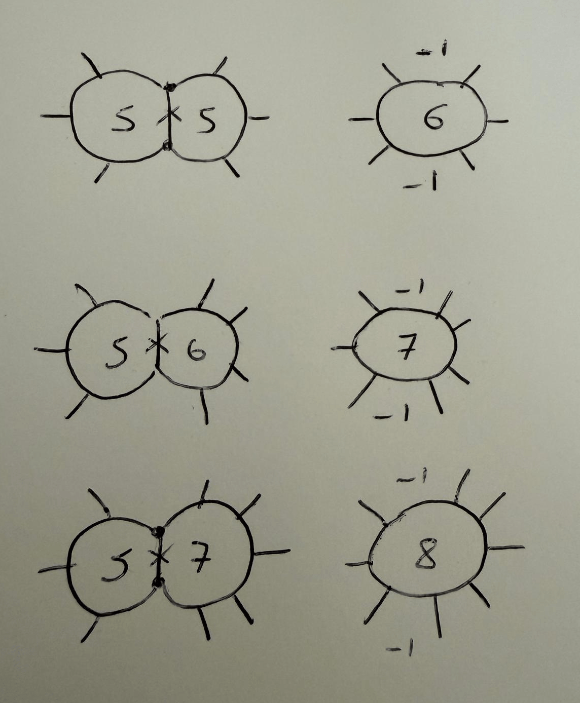
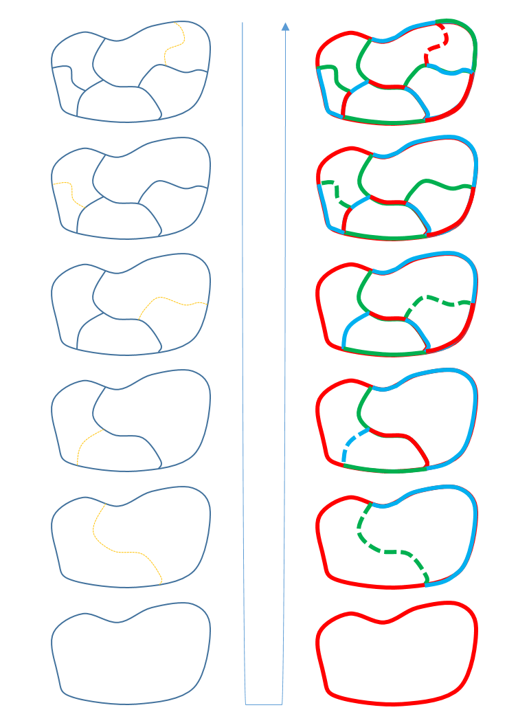
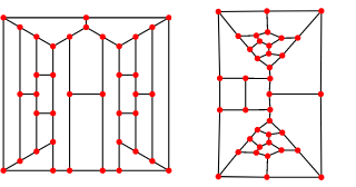
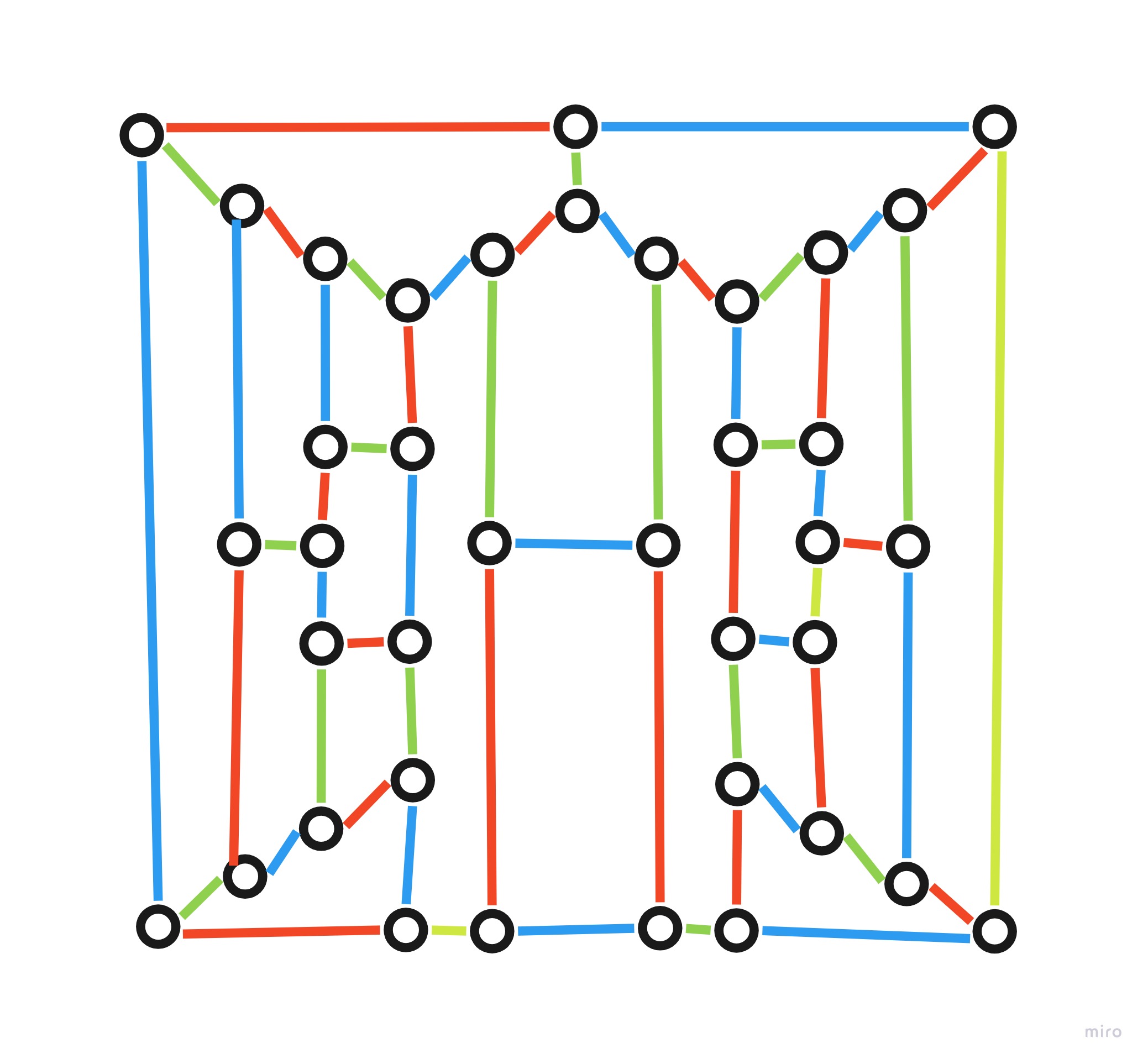
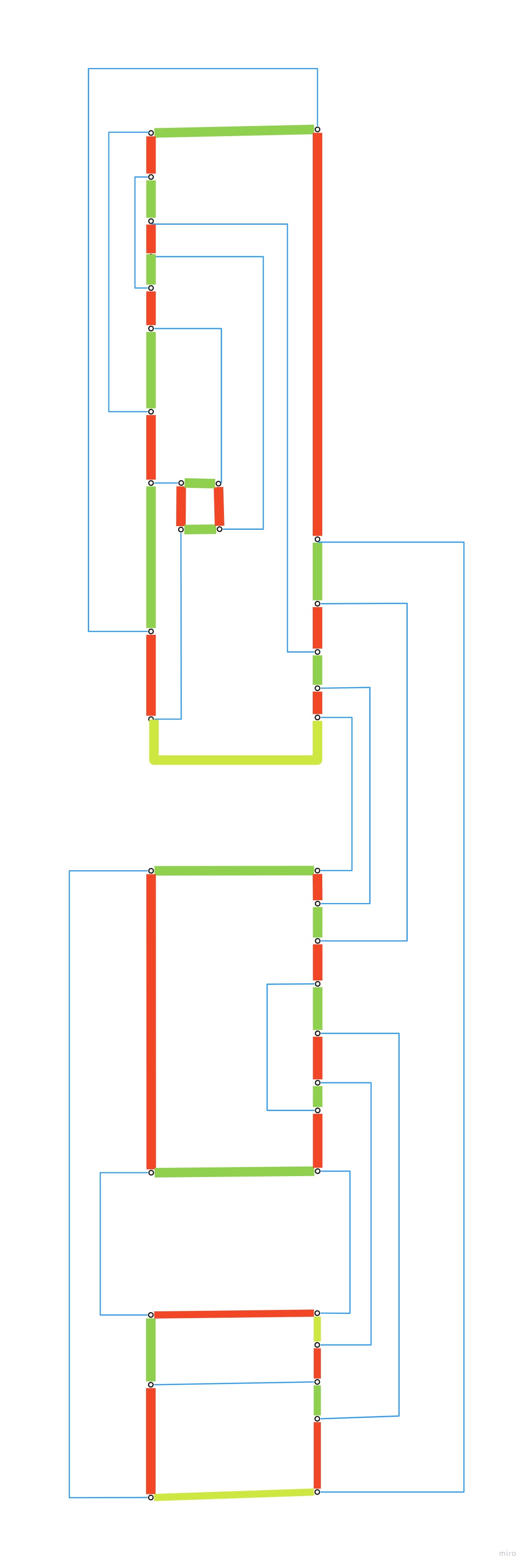
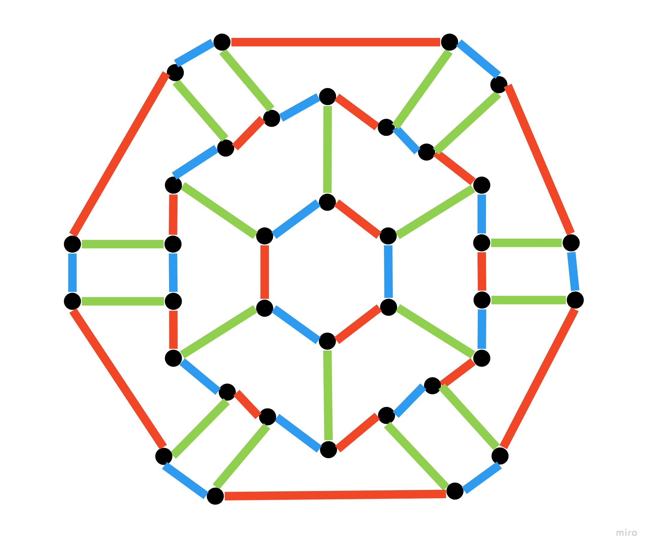
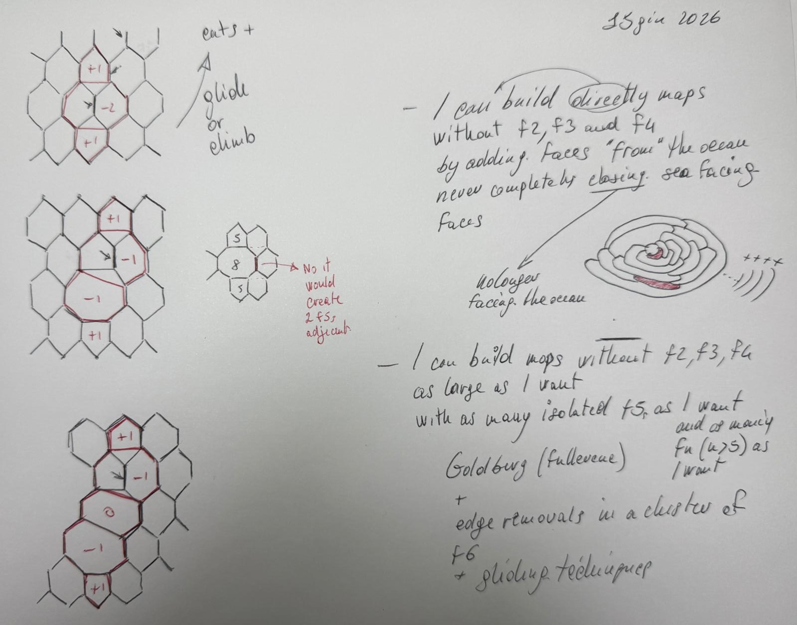
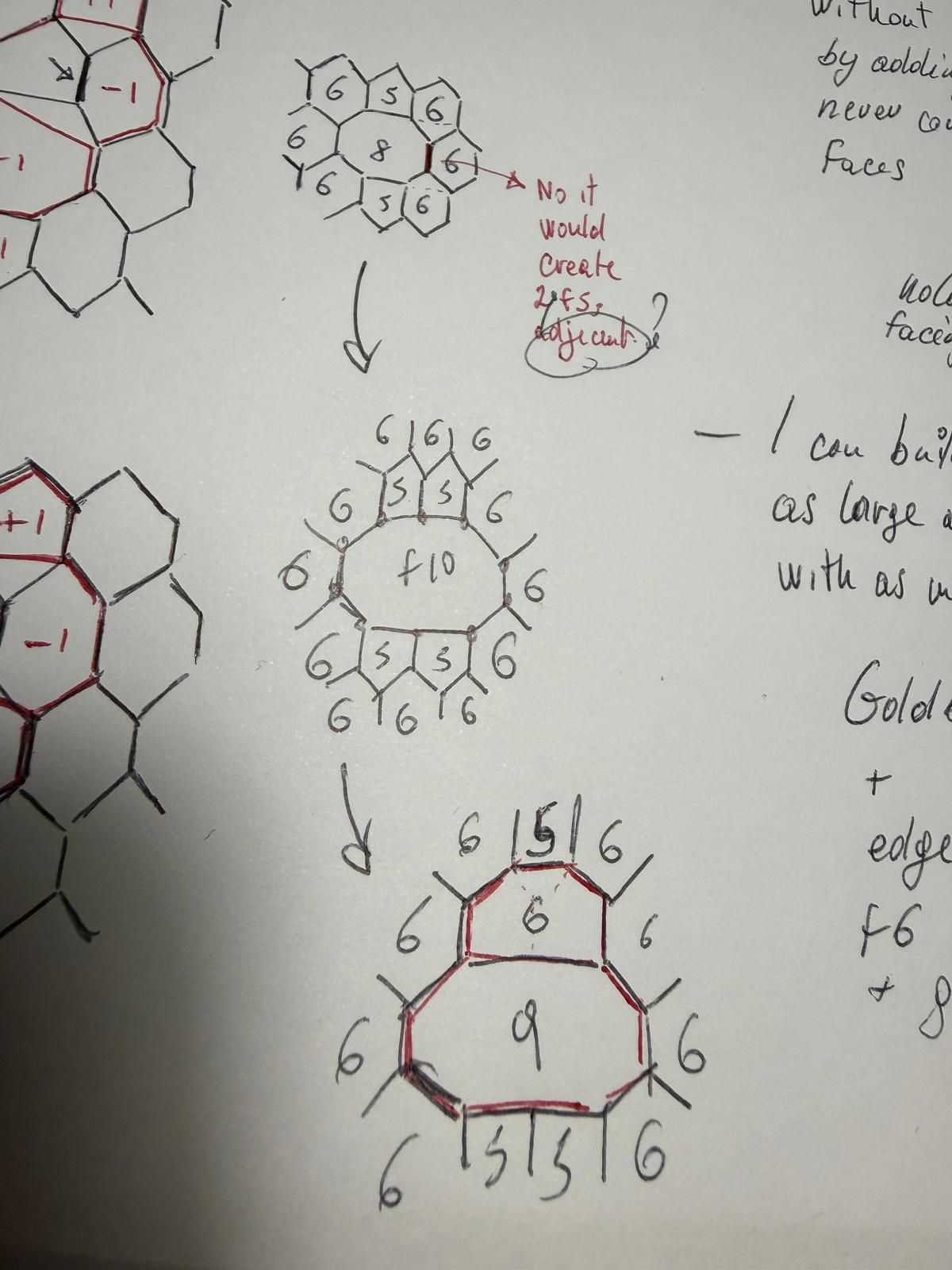
The basic act of surgery is brutal and simple: delete one edge together with its two endpoints, and smooth the two resulting degree-two corners. Four faces feel it. The two faces that shared the edge merge into one face of size a+b−4 (6+6−4=8 sides); the two flanking hexagons drop to pentagons. This is the famous 5-8-5 defect of graphene physics (a reconstructed divacancy: two missing atoms) Volterra studied. Net charge: +1−2+1=0. Crucially, the surrounding ring of hexagons is combinatorially untouched. The defect is invisible from one ring away.

From there, the whole game is choosing the right edge so that the F5 face glides over the ocean to be kept as isolated as wanted.


I was already familiar with Paul Wernicke and Philip Franklin, who hunted the Four Color Theorem by proving unavoidability results: in any cubic spherical map with all faces of size at least five, some pentagon must sit next to a face of size at most six (Wernicke), in fact, next to two such faces (Franklin). Their method, discharging, the art of letting positive charge flow along edges until a contradiction surfaces, is the ancestor of the 1976 computer proof of the Four Color Theorem.

Victor Eberhard, a German geometer who lost his sight as a young man and did all of this work blind, proved in 1891 that any face-count sequence satisfying the law of twelve can be realized by an actual polyhedron, provided you are allowed to throw in enough neutral hexagons. Eberhard’s theorem is the existential backbone of everything here: the hexagons are the silent majority that makes any charge distribution geometrically possible

Vito Volterra, the great Italian analyst, supplied the deepest tool without knowing it. His theory of distorsioni in elastic bodies, cut the material, shift one lip of the cut by a lattice step, re-glue, is exactly the theory of dislocations that crystallographers and graphene physicists use today. On a hexagonal map, a Volterra cut-and-shift leaves a pentagon at one end of the seam and a heptagon at the other, with unharmed hexagons everywhere in between: a +1+1 and a -1-1, created in pairs, separable at will.

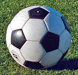
Michael Goldberg classified the highly symmetric cubic maps made of twelve pentagons and any number of hexagons, the Goldberg polyhedra, rediscovered by chemists as fullerenes and by virologists in virus capsids. A giant Goldberg map is the perfect blank canvas: a near-infinite sea of neutral hexagons with twelve pentagonal hills parked at the corners of an icosahedron, as far from each other as you please.

Learn from previously colored maps


Stay with me 👀, because this is going to like you.

I came up with an idea that feels so simple and obvious that I can’t help but wonder why I hadn’t thought of it earlier. Maybe difficult to implement 😭 but the idea it is good and simple.

I’m curious if anyone has explored something similar, or if there are known related results 🤔

Would love to hear your thoughts!

I’ve been working on the Four Color Theorem 🎨, specifically on reducing planar 3-regular graphs down to a minimal configuration and then back reconstructing them step by step using, when necessary, different color Kempe chain switches techniques.

The challenge is that while my reduction strategy works in most cases ✅, there are configurations where the reconstruction gets stuck ❌ and Kempe switches don’t resolve the conflict. Only by shuffling the order of face selection 🔀 I’ve always been able to eventually color the map.

Here’s the idea 🚀: instead of trying to design the perfect reduction strategy upfront, why not start from the opposite direction?

Since I can already color arbitrarily complex graphs (even if it requires trial, backtracking, and random Kempe switches 🎲), I can treat successful colorings as “ground truth”.

From there, I can analyze the sequence of reductions on an already colored graph and observe which choices preserve a valid path back to a full coloring 🔍

In other words, rather than guessing the best reduction strategy, I can learn it from examples of graphs that have already been four-colored.

Let’s leave the beach: pentagonal regions and the Four Color Theorem (2/2)


F5-Fn

Case F5-F5

By removing an edge between two F5 faces, you obtain an F6 face. The two adjacent faces that shared the removed vertices each lose one edge. If the two adjacent faces are actually the same face, the number of edges decreases by two.

General case F5-Fn

By removing an edge between an F5 face and a Fn face, you obtain an F(n+1) face. The two adjacent faces that shared the removed vertices each lose one edge. If the two adjacent faces are actually the same face, the number of edges decreases by two.

The problem is that maps on the sphere can exist:

Let’s go to the beach: pentagonal regions and the Four Color Theorem


I need relax. Let’s go to the beach!

Personal note: I don’t know where I am headed, so don’t follow me. I am just wandering around taking notes.

Suppose that there exist maps that are not four-colorable, perhaps only one, perhaps a few, or even infinitely many.

Now, remove from this set all maps that have regions with 2, 3, or 4 borders. For the scope of the four color theorem and without lack of generality, we can skip them. 🤞🏻 I am confident it is true, but not completely sure I can do this step of removing these maps with no further considerations. Or at least it should be proved.

Now select a pentagonal region and regard it as the outer boundary: the ocean that surrounds all other lands.

And now walk along the shoreline.

What can we say about the five regions that face the ocean?

Can one of them be always an F5?

The answer is no, not always. Fullerene graphs show that it is possible for all F5 faces to be isolated, with no two pentagons sharing an edge. The standard example is the Buckminsterfullerene. Or, more commonly a soccer ball.

C60

Can one of them be always an F6?

Euler’s formula neither guarantees nor rules out this possibility.

1 F5 – 0 F6 – 1 F7 – 2 F8 – 3 F9 – … = 12

👉 I don’t know if there are studies done to analyze these maps. F5 always surrounded by F7 or higher.

To be continued …

  • Remove an edge between F5-F5, or F5-F6 or 😦 F5-F7+
  • Analyze all combinations of colors along the new shoreline of the reduced maps, and search for a contradiction to the hypothesis that there exist maps that cannot be colored with four colors

Boosting performance: Sage to Python/Networkx transition


I converted the Sage implementation to a pure Python / Networkx solution.

  • sage 4ct.py -r 2000
  • python3 4ct_without_sage.py -r 2000
SagePython3 + Networkx
Random graph creation17 min 59 s
* RandomTriangulation
22 s
* Custom
Planar embedding16 min 09 s
* dual + set_embedding=True
0 s
* Not necessary
Elaboration2 min 12 s1 min 58 s

Here is the file:

Other run:

  • sage 4ct.py -r 1000
  • python3 4ct_without_sage.py -r 1000
SagePython3 + Networkx
Random graph creation3 min 19 s6 s
Planar embedding2 min 44 s0 s
Elaboration14 s23 s

Optimizing Graph Coloring with Reinforcement Learning


This is what I will be working for a while. Restart is difficult, but necessary.

Why use Reinforcement Learning for Graph coloring?

In my Python application, that works on 3-regular planar graph, deciding which is the order of the edges to remove can be non-trivial. A naive approach randomly picks edges from F2 faces, F3, F4 or F5. This is the approach I used :-(. It leads to impasses when rebuilding the map. See https://4coloring.wordpress.com/2014/08/27/four-color-theorem-experimenting-impasses-as-in-life/

But a reinforcement learning agent can learn to make better selections over time to reduce color conflicts, I hope :-), and shed light on some properties of the graph that can be used in the proof.

The code will be here: https://github.com/stefanutti/maps-coloring-python

Remove one edge at a time from F2, F3, F4, or F5 faces. These faces represent the basic unavoidable set. This process will reduce the map to three faces, including the ocean as the external area. Afterward, I will restore the edges in reverse order, consistently working with 3-regular planar graphs. I will consider Tait coloring of the edges and apply, when necessary, Kempe’s chain color switching to the edges.

Remove edges a then restore them

For the Agent:

  • Environment initialization = The starting uncolored 3-regular planar graphs
  • Action = Select the edge to remove from the 3-regular planar graphs
  • State = The updated 3-regular planar graphs
  • Reward = +1 if Random Kempe’s chain color switching was not necessary, -1 otherwise

4CT and loops, cycles, circuits, chains, paths


I realized that for some posts I may have used “Kempe loops” and “Kempe cycles” to describe closed “Kempe chains”, that in other words form closed paths (cycles). I think it would have been better always to use “Kempe cycles”.

https://en.wikipedia.org/wiki/Loop_(graph_theory)

https://en.wikipedia.org/wiki/Path_(graph_theory)

https://en.wikipedia.org/wiki/Hamiltonian_path

Non-Hamiltonian 3-regular planar graphs, Tait coloring and Kempe cycles … what else ;-)


Considering the smallest known non-Hamiltonian 3-regular planar graphs, discovered by Barnette-Bosák-Lederberg, I computed the Tait coloring and then deformed it to put in evidence the R-G cycles that in this case are four.

Links to the historical importance of this graph:

https://mathworld.wolfram.com/Barnette-Bosak-LederbergGraph.html

https://en.wikipedia.org/wiki/Barnette–Bosák–Lederberg graph

And here is the Tait coloring of this graph:

Deformed here to better show the R-G cycles:

Tait coloring and the four color theorem: personal Q&A


Some questions about the previous post:

Q1) Can cycles be concentric?

Yes, see this example.

Q2) Verify if at least one of the cycles (R-G, R-B, or G-B) form an Hamiltonian circuit

False.

From the Tait’s conjecture we now know (now = 1946 by William Thomas Tutte) that 3-regular graphs exist also without an Hamiltonian circuit. It means that, no matter what, it is not possible to find a cycle that touches all vertices, and therefore no single Kempe cycles of any two color selection, can exist.

From Wikipedia, the free encyclopedia

This article is about graph theory. For the conjectures in knot theory, see Tait conjectures.

In mathematics, Tait’s conjecture states that “Every 3-connected planar cubic graph has a Hamiltonian cycle (along the edges) through all its vertices“. It was proposed by P. G. Tait (1884) and disproved by W. T. Tutte (1946), who constructed a counterexample with 25 faces, 69 edges and 46 vertices. Several smaller counterexamples, with 21 faces, 57 edges and 38 vertices, were later proved minimal by Holton & McKay (1988). The condition that the graph be 3-regular is necessary due to polyhedra such as the rhombic dodecahedron, which forms a bipartite graph with six degree-four vertices on one side and eight degree-three vertices on the other side; because any Hamiltonian cycle would have to alternate between the two sides of the bipartition, but they have unequal numbers of vertices, the rhombic dodecahedron is not Hamiltonian. The conjecture was significant, because if true, it would have implied the four color theorem: as Tait described, the four-color problem is equivalent to the problem of finding 3-edge-colorings of bridgeless cubic planar graphs. In a Hamiltonian cubic planar graph, such an edge coloring is easy to find: use two colors alternately on the cycle, and a third color for all remaining edges. Alternatively, a 4-coloring of the faces of a Hamiltonian cubic planar graph may be constructed directly, using two colors for the faces inside the cycle and two more colors for the faces outside.

Smallest known non-Hamiltonian 3-regular planar graph: https://mathworld.wolfram.com/Barnette-Bosak-LederbergGraph.html.

Next post will be on the four coloring of the barnette-bosák-lederberg graph, which is the smallest known non-Hamiltonian graph, and the analysis of its Kempe cycles.

Q3) What about if I start with finding cycles, of even length (# of edges), that cross all vertices?

Some initial considerations: If cycles have to fit with Kempe cycles (closed paths of two alternating colors), they have to be of even length, and that would also mean that the total number of vertices crossed by all the cycles of the same two colors should be even too. Is it like this, or am I missing something? What about graphs with an odd number of vertices? Am I missing something?

Answer to the initial consideration: https://math.stackexchange.com/questions/181833/proving-that-the-number-of-vertices-of-odd-degree-in-any-graph-g-is-even + https://math.stackexchange.com/questions/181833/proving-that-the-number-of-vertices-of-odd-degree-in-any-graph-g-is-even

Finding cycles seems to be as difficult as finding a solution for of 4 coloring problem 😦