There are some methods around to create planar graphs. One of these is based on the Delaunay triangulation algorithm from which you can derive its dual, a 3 regular planar graph. Tools and libraries that I found around (sage, networkx and others), permits you to save the graph using one of common format to represent the graph itself, specifically: .dot, .graphml, .GEXF, .gpickle and others). One problem that I found is that if I save the graph I loose the planar representation of it.

Since for what I am trying to do, namely demonstrate with pencil and paper that the four color theorem has a simpler demonstration, I need to work directly with the planar representation of the graph.

I decided to implement my own method (based on edge addition to planar graphs. See “John M. Boyer and Wendy J. Myrvold, On the Cutting Edge: Simplified O(n) Planarity by Edge Addition. Journal of Graph Algorithms and Applications, Vol. 8, No. 3, pp. 241-273, 2004.”) to generate an save the graph directly using its planar representation. Get the code here at: https://github.com/stefanutti/maps-coloring-python. The program generates random planar graphs without using graphs library and most importantly without using complex algorithms, as planar embedding or planarity testing.

Planar embedding: “A combinatorial embedding of a graph is a clockwise ordering of the neighbors of each vertex. From this information one can define the faces of the embedding”.

sage: T = graphs.TetrahedralGraph()
sage: T.faces({0: [1, 3, 2], 1: [0, 2, 3], 2: [0, 3, 1], 3: [0, 1, 2]})
[[(0, 1), (1, 2), (2, 0)],
[(3, 2), (2, 1), (1, 3)],
[(3, 0), (0, 2), (2, 3)],
[(3, 1), (1, 0), (0, 3)]]

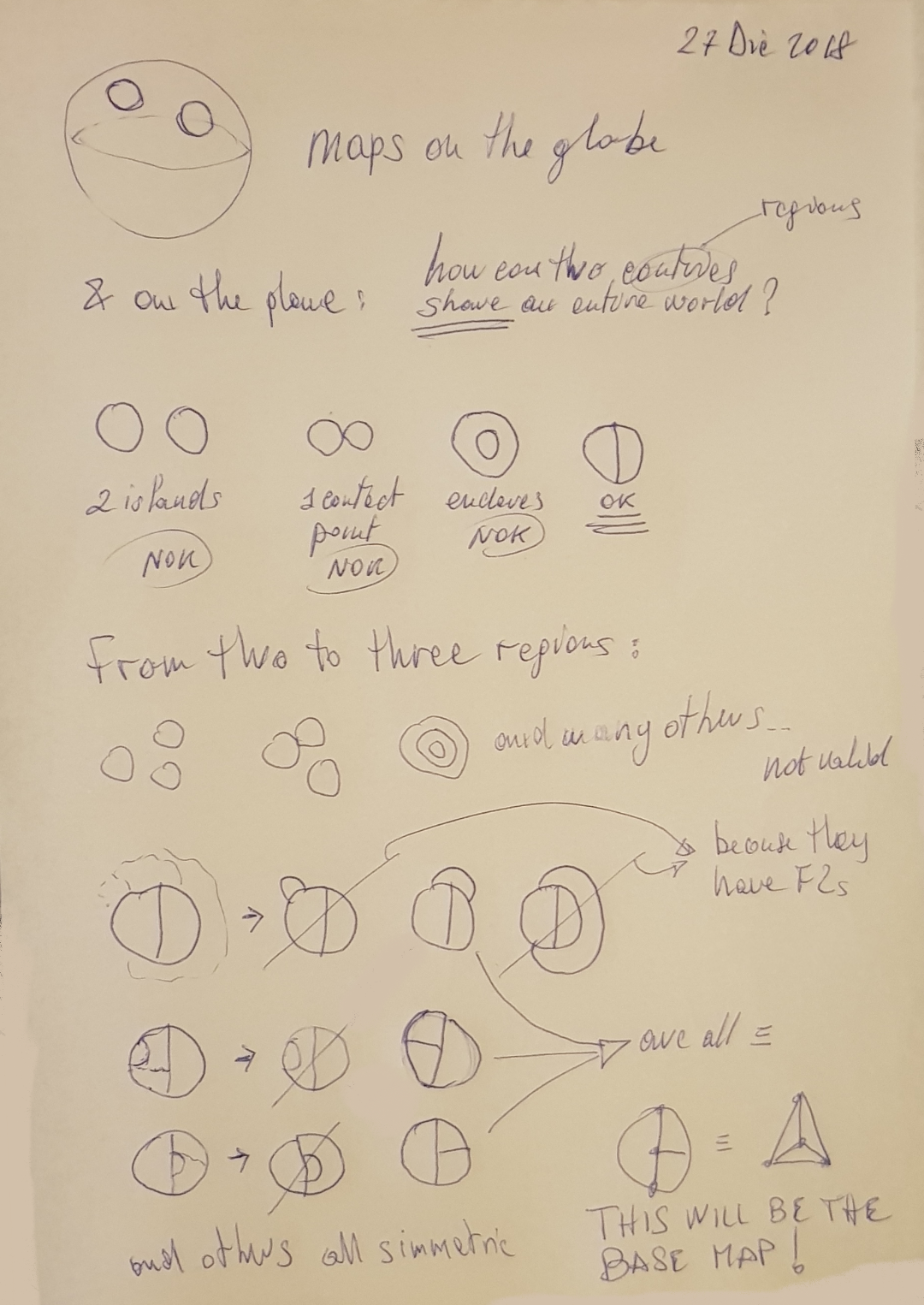
Edge addition can start from a basic graph of four faces (bottom right). In the third last line of this picture I added edges from a graph with 3 faces and 2 vertices (considering the ocean). But as you can deduct from the other pictures I can safely start from a graph with 4 faces and 4 vertices (bottom right).