Euler’s formula at work


During the process of removing faces from a planar map (cubic planar graph) this video shows how the Euler’s equation redistribute its weights:

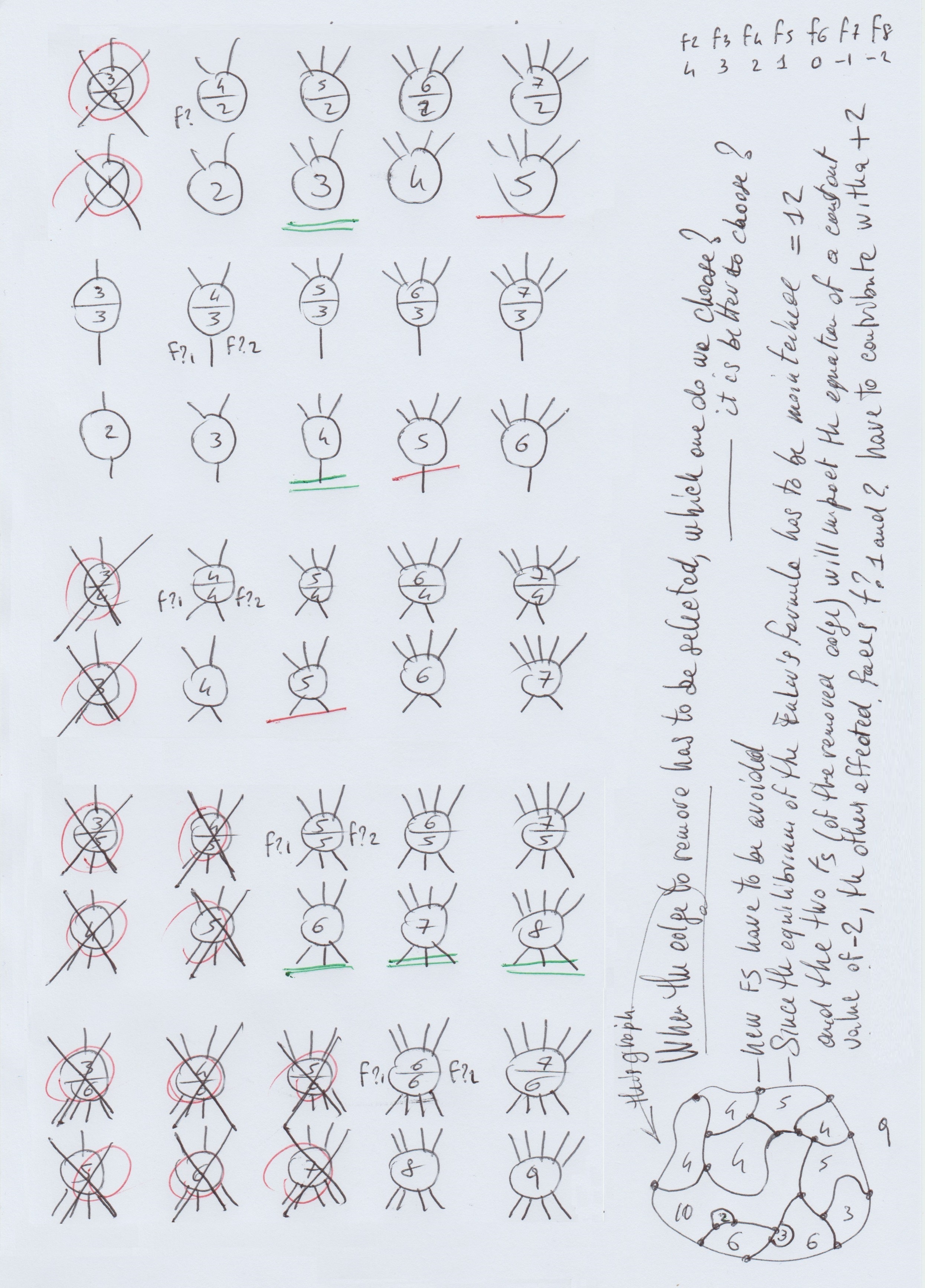
+4F2 +3F3 +2F4 +1F5 +0F6 -1F7 -2F8 -3F9 …. = 12

The map that has been used to produce this video is represented by a planar cubic graph made of almost 10000 faces (20000 vertices and 27972 edges).

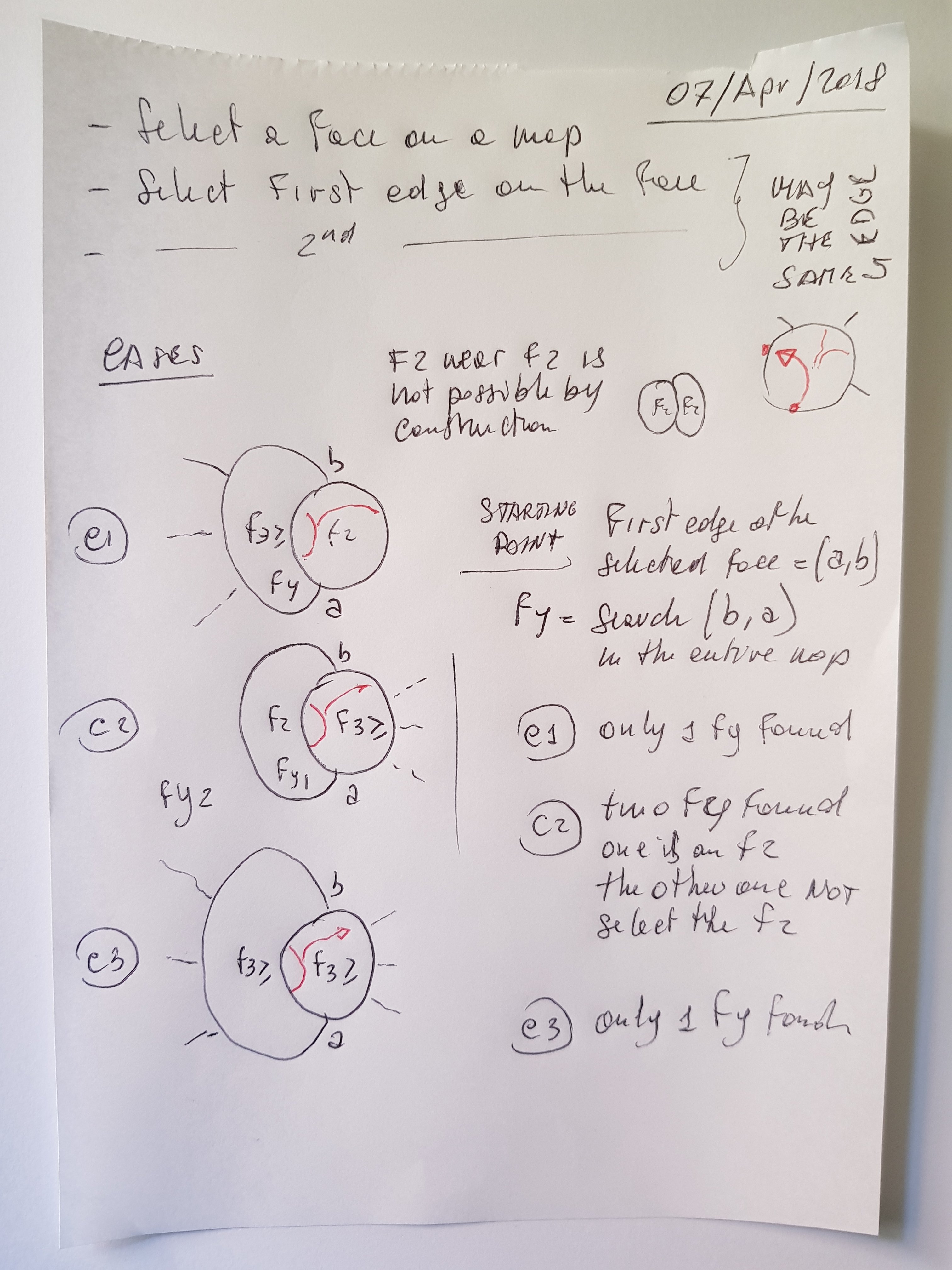
The selection for the edges to remove that I used was: take an edge from an F2. Then, if no F2 exist, use an F3. And then, if no F3 exist, use an F4 and finally an F5.

A graph with 20000 vertices opened by Gephy appears as a black square 😦

Here is the .dot file and the planar representation of the map.

Return it to me Tait coloured if you can 🙂

mailto:mario.stefanutti@gmail.com?subject=4CT Tait coloring

Meaning with all edges using only three colours (without conflicts at the vertices), which is equivalent to color the faces with four colours.

Bye

PS:

2020-04-26 22:37:21,310 - root - INFO - ------------------
2020-04-26 22:37:21,310 - root - INFO - BEGIN: Print stats
2020-04-26 22:37:21,310 - root - INFO - ------------------
2020-04-26 22:37:21,311 - root - INFO - Stat: CASE-F2-01 = 4114
2020-04-26 22:37:21,311 - root - INFO - Stat: CASE-F3-01 = 4478
2020-04-26 22:37:21,311 - root - INFO - Stat: CASE-F4-01 = 732
2020-04-26 22:37:21,311 - root - INFO - Stat: CASE-F4-02 = 442
2020-04-26 22:37:21,311 - root - INFO - Stat: CASE-F4-03 = 231
2020-04-26 22:37:21,311 - root - INFO - Stat: CASE-F5-C1!=C2-SameKempeLoop-C1-C2 = 1
2020-04-26 22:37:21,311 - root - INFO - Stat: CASE-F5-C1==C2-SameKempeLoop-C1-C3 = 1
2020-04-26 22:37:21,312 - root - INFO - Stat: CASE-F5-C1==C2-SameKempeLoop-C1-C4 = 0
2020-04-26 22:37:21,312 - root - INFO - Stat: MAX_RANDOM_KEMPE_SWITCHES = 0
2020-04-26 22:37:21,312 - root - INFO - Stat: TOTAL_RANDOM_KEMPE_SWITCHES = 0
2020-04-26 22:37:21,312 - root - INFO - Stat: time_ELABORATION = 1015
2020-04-26 22:37:21,312 - root - INFO - Stat: time_ELABORATION_BEGIN = Sun Apr 26 22:19:55 2020
2020-04-26 22:37:21,313 - root - INFO - Stat: time_ELABORATION_END = Sun Apr 26 22:36:50 2020
2020-04-26 22:37:21,313 - root - INFO - Stat: time_GRAPH_CREATION_BEGIN = Sun Apr 26 22:19:22 2020
2020-04-26 22:37:21,313 - root - INFO - Stat: time_GRAPH_CREATION_END = Sun Apr 26 22:19:55 2020
2020-04-26 22:37:21,313 - root - INFO - ----------------
2020-04-26 22:37:21,314 - root - INFO - END: Print stats
2020-04-26 22:37:21,314 - root - INFO - ----------------

Zoom on a planar graph, 10000 nodes, three-edge Tait colored


I generated a planar map of 10000 nodes and then colored using the 4ct python coloring program.

It did use Tait coloring (3-edge-coloring) which is equivalent to the four face coloring of the four color theorem.

It works pretty fast using:

  • graph reduction removing edges from F2, F3, F4, F5
  • graph rebuilding using Kempe chain color switching techniques

The globe and the four color theorem


The four color theorem appeared in 1852, talking about the problem of coloring real maps. Let’s examine some basic aspects of these maps in relation to the four color theorem.

A world with just water and one land with no divisions, topologically equivalent to a disk, needs only two colors to paint the land and the ocean. This is the beginning, as the Pangea on Earth long ago.

If two parties want to share this land and both want to have access to the ocean and have contiguous regions, there is only one possible configuration, and the resulting map can be represented by a planar graph with 2 vertexes and 3 edges (multiedge graph). The other solutions that have been excluded by the two restrictions: “have access to the ocean” and “contiguous regions” are not so interesting for the scope of the theorem (see previous post).

If a third party comes into play, the initial region (surrounded by the ocean) has to be split among three parties, with the same two restrictions as stated before: “have access to the ocean” and “be contiguous regions”. If we consider all possible combinations, we can also see that among them there are some that can be eliminated introducing a third rule: “all faces have to touch each other”. This third rule can be added because all the configurations in which the three faces don’t touch each other contain F2 faces and therefore (is it to be proved?) can be eliminated. It will then rest only one configuration that meet all criteria, that is the one printed at the bottom right of the previous post image.

Generate planar graphs


There are some methods around to create planar graphs. One of these is based on the Delaunay triangulation algorithm from which you can derive its dual, a 3 regular planar graph. Tools and libraries that I found around (sage, networkx and others), permits you to save the graph using one of common format to represent the graph itself, specifically: .dot, .graphml, .GEXF, .gpickle and others). One problem that I found is that if I save the graph I loose the planar representation of it.

Since for what I am trying to do, namely demonstrate with pencil and paper that the four color theorem has a simpler demonstration, I need to work directly with the planar representation of the graph.

I decided to implement my own method (based on edge addition to planar graphs. See “John M. Boyer and Wendy J. Myrvold, On the Cutting Edge: Simplified O(n) Planarity by Edge Addition. Journal of Graph Algorithms and Applications, Vol. 8, No. 3, pp. 241-273, 2004.”) to generate an save the graph directly using its planar representation. Get the code here at: https://github.com/stefanutti/maps-coloring-python. The program generates random planar graphs without using graphs library and most importantly without using complex algorithms, as planar embedding or planarity testing.

Planar embedding: “A combinatorial embedding of a graph is a clockwise ordering of the neighbors of each vertex. From this information one can define the faces of the embedding”.

sage: T = graphs.TetrahedralGraph()
sage: T.faces({0: [1, 3, 2], 1: [0, 2, 3], 2: [0, 3, 1], 3: [0, 1, 2]})
[[(0, 1), (1, 2), (2, 0)],
[(3, 2), (2, 1), (1, 3)],
[(3, 0), (0, 2), (2, 3)],
[(3, 1), (1, 0), (0, 3)]]

Edge addition can start from a basic graph of four faces (bottom right). In the third last line of this picture I added edges from a graph with 3 faces and 2 vertices (considering the ocean). But as you can deduct from the other pictures I can safely start from a graph with 4 faces and 4 vertices (bottom right).

Four color theorem: A fast algorithm – 2


Four color theorem: A fast algorithm

These are the OLD and NEW (last column) execution times on my new laptop:

  • 100 – 196 vertices, 294 edges = 0 seconds – 0 seconds
  • 200 – 396 vertices, 594 edges = 1 seconds – 0 seconds
  • 300 – 596 vertices, 894 edges = 4 seconds – 1 second
  • 400 – 796 vertices, 1194 edges = 6 seconds – 1 second
  • 500 – 996 vertices, 1494 edges = 8 seconds – 2 seconds
  • 600 – 1196 vertices, 1794 edges = 10 seconds – 4 seconds
  • 700 – 1396 vertices, 2094 edges = 16 seconds – 6 seconds
  • 800 – 1596 vertices, 2394 edges = 18 seconds – 7 seconds
  • 900 – 1796 vertices, 2694 edges = 22 seconds – 9 seconds
  • 1000 – 1996 vertices, 2994 edges = 26 seconds – 11 seconds

Four color theorem: about edges selection


For the decomposition of a graph representing a map, I’m trying to use different algorithms to select the edge to remove.

The question is:

  • When you have multiple valid choices, which is the best edge to select … if any?

Some basic rules are:

  • Avoid new F5 to be created
  • Get rid of F5 whenever is possible, selecting the edge of a face with 2, 3 or 4 edges
  • Consider to remove an edge from an F5 face only if no faces with 2, 3, 4 edges exist

Here are all possibilities. Last 2 groups (removing edges from F5 and F6) don’t have to be taken into account. I just wanted to see how it continued after the cases with faces made of 2, 3, 4 and 5 edges:

edges-selection-possibilities