I realized that for some posts I may have used “Kempe loops” and “Kempe cycles” to describe closed “Kempe chains”, that in other words form closed paths (cycles). I think it would have been better always to use “Kempe cycles”.
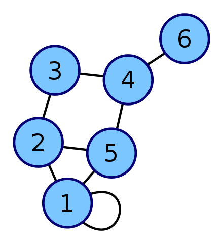
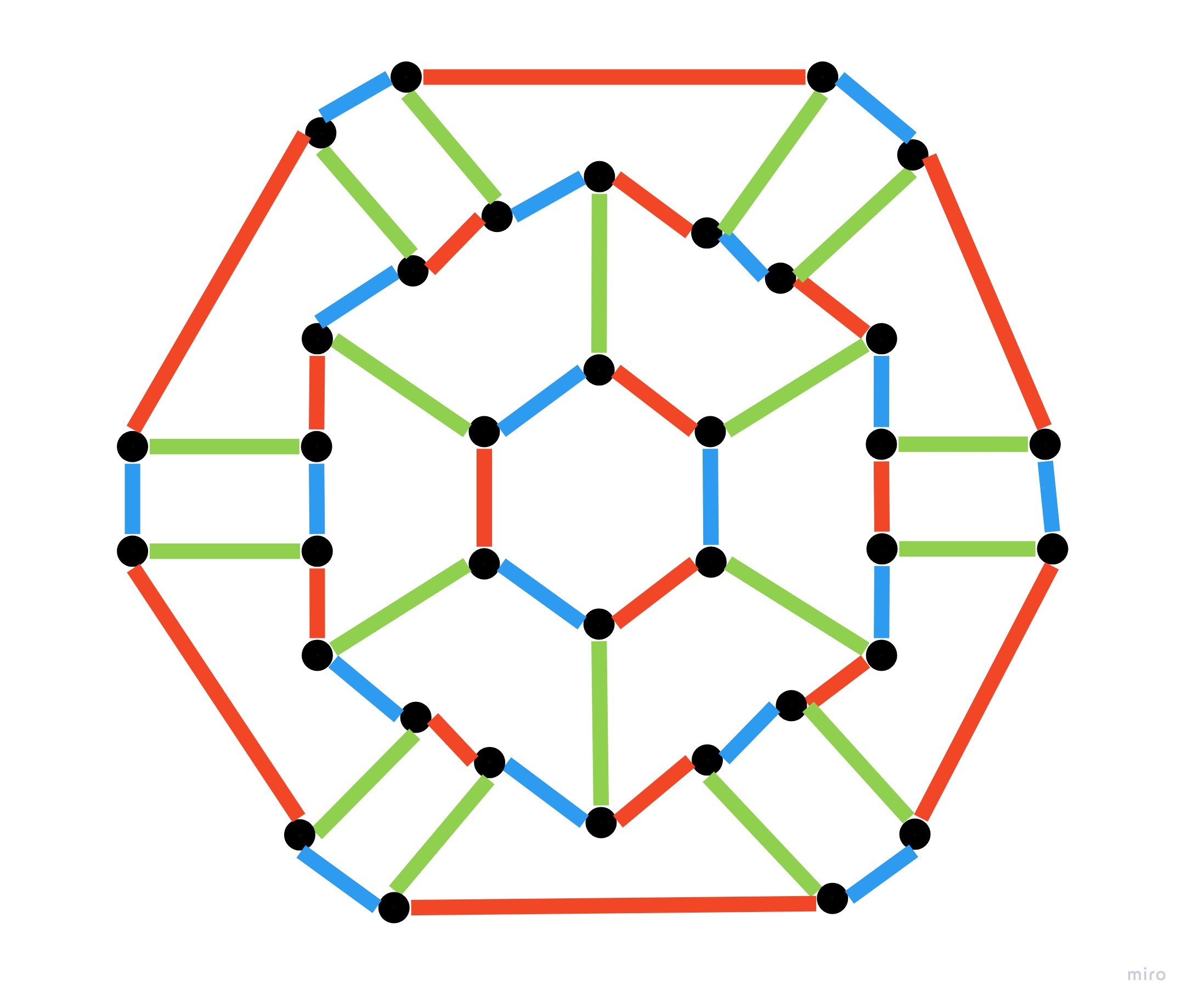
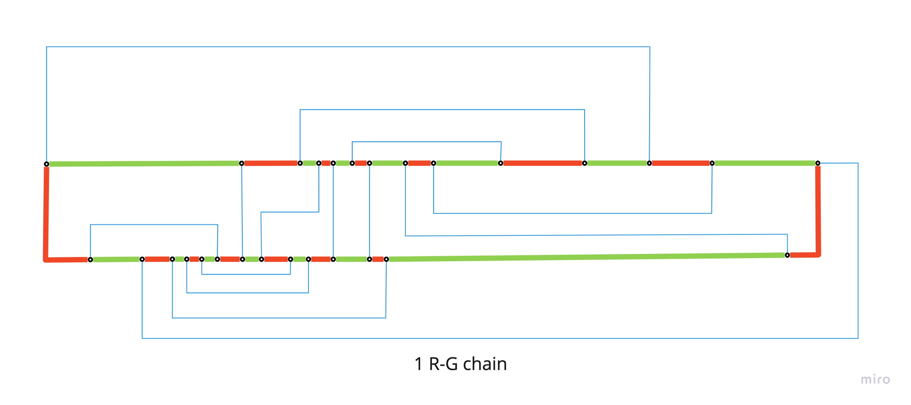
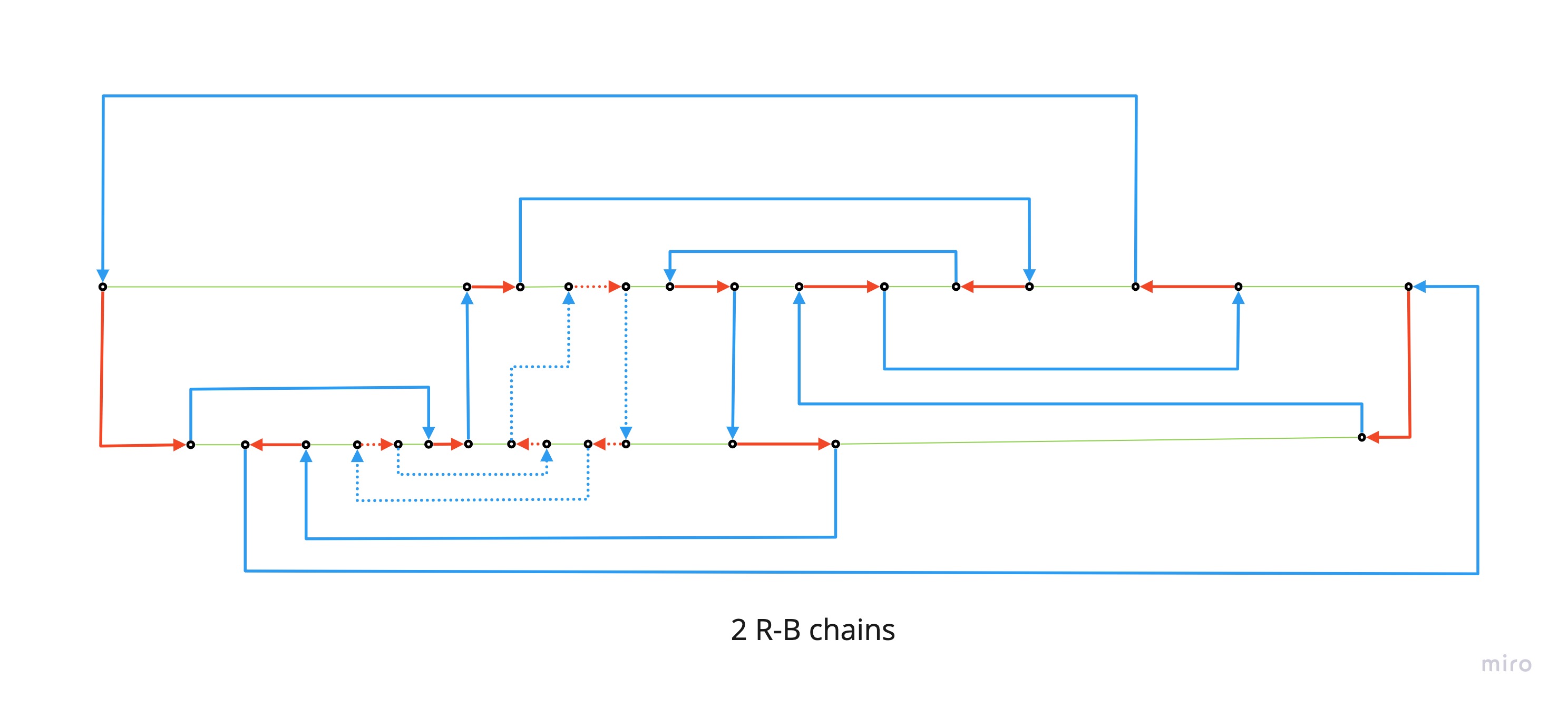
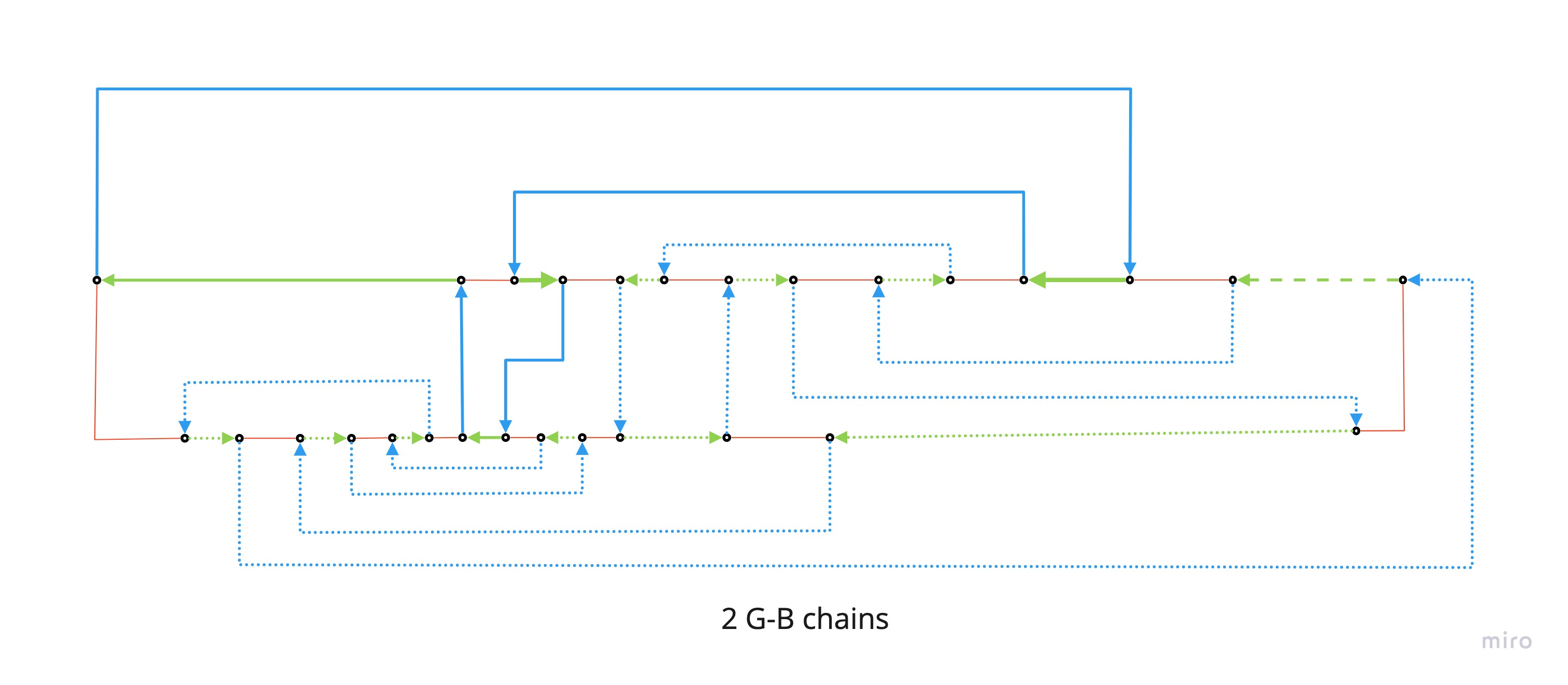
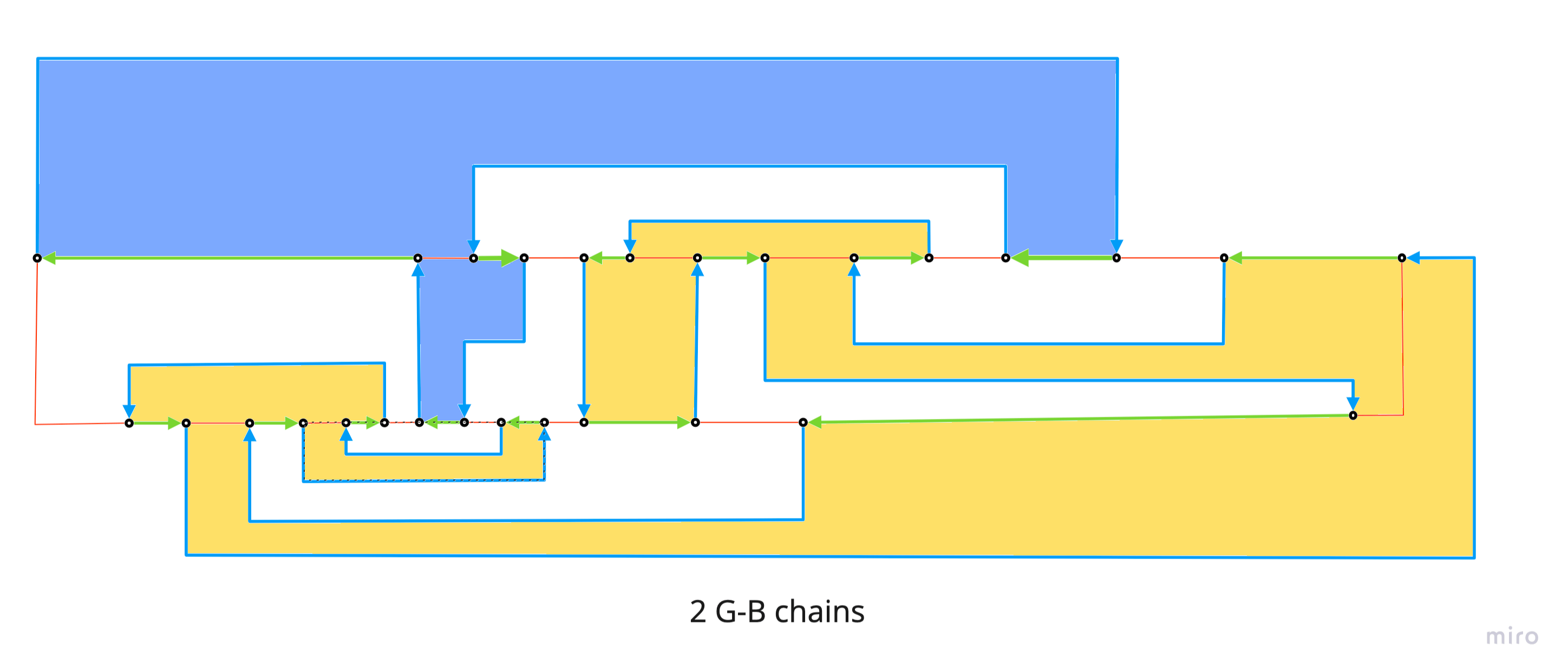
Considering the smallest known non-Hamiltonian 3-regular planar graphs, discovered by Barnette-Bosák-Lederberg, I computed the Tait coloring and then deformed it to put in evidence the R-G cycles that in this case are four.
Q2) Verify if at least one of the cycles (R-G, R-B, or G-B) form an Hamiltonian circuit
False.
From the Tait’s conjecture we now know (now = 1946 by William Thomas Tutte) that 3-regular graphs exist also without an Hamiltonian circuit. It means that, no matter what, it is not possible to find a cycle that touches all vertices, and therefore no single Kempe cycles of any two color selection, can exist.
From Wikipedia, the free encyclopedia
This article is about graph theory. For the conjectures in knot theory, see Tait conjectures.
In mathematics, Tait’s conjecture states that “Every 3-connectedplanarcubic graph has a Hamiltonian cycle (along the edges) through all its vertices“. It was proposed by P. G. Tait (1884) and disproved by W. T. Tutte (1946), who constructed a counterexample with 25 faces, 69 edges and 46 vertices. Several smaller counterexamples, with 21 faces, 57 edges and 38 vertices, were later proved minimal by Holton & McKay (1988). The condition that the graph be 3-regular is necessary due to polyhedra such as the rhombic dodecahedron, which forms a bipartite graph with six degree-four vertices on one side and eight degree-three vertices on the other side; because any Hamiltonian cycle would have to alternate between the two sides of the bipartition, but they have unequal numbers of vertices, the rhombic dodecahedron is not Hamiltonian. The conjecture was significant, because if true, it would have implied the four color theorem: as Tait described, the four-color problem is equivalent to the problem of finding 3-edge-colorings of bridgeless cubic planar graphs. In a Hamiltonian cubic planar graph, such an edge coloring is easy to find: use two colors alternately on the cycle, and a third color for all remaining edges. Alternatively, a 4-coloring of the faces of a Hamiltonian cubic planar graph may be constructed directly, using two colors for the faces inside the cycle and two more colors for the faces outside.
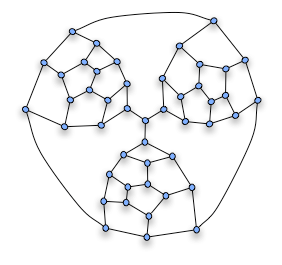
Next post will be on the four coloring of the barnette-bosák-lederberg graph, which is the smallest known non-Hamiltonian graph, and the analysis of its Kempe cycles.
Q3) What about if I start with finding cycles, of even length (# of edges), that cross all vertices?
Some initial considerations: If cycles have to fit with Kempe cycles (closed paths of two alternating colors), they have to be of even length, and that would also mean that the total number of vertices crossed by all the cycles of the same two colors should be even too. Is it like this, or am I missing something? What about graphs with an odd number of vertices? Am I missing something?
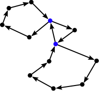
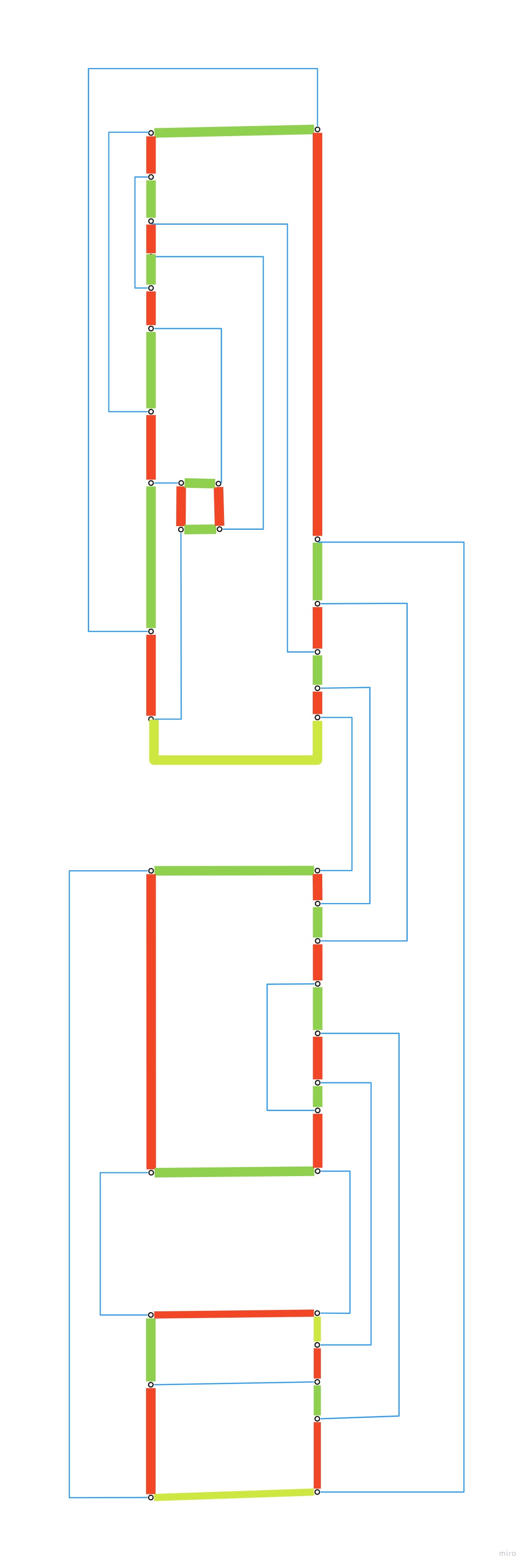
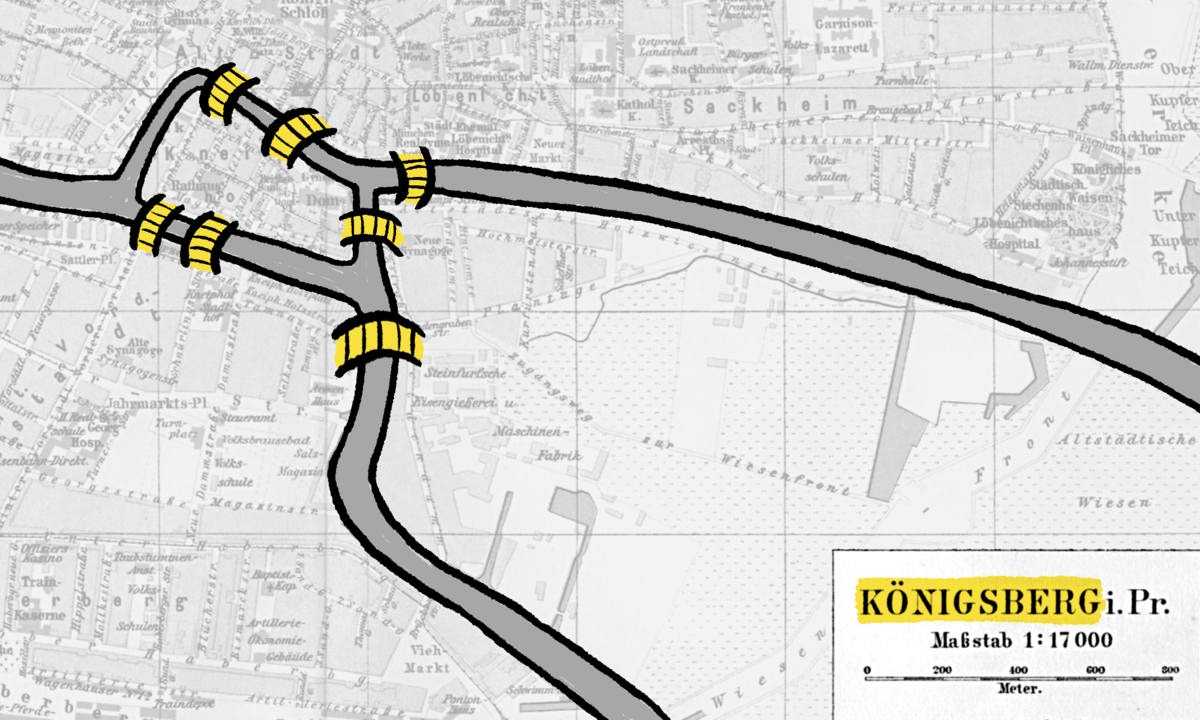
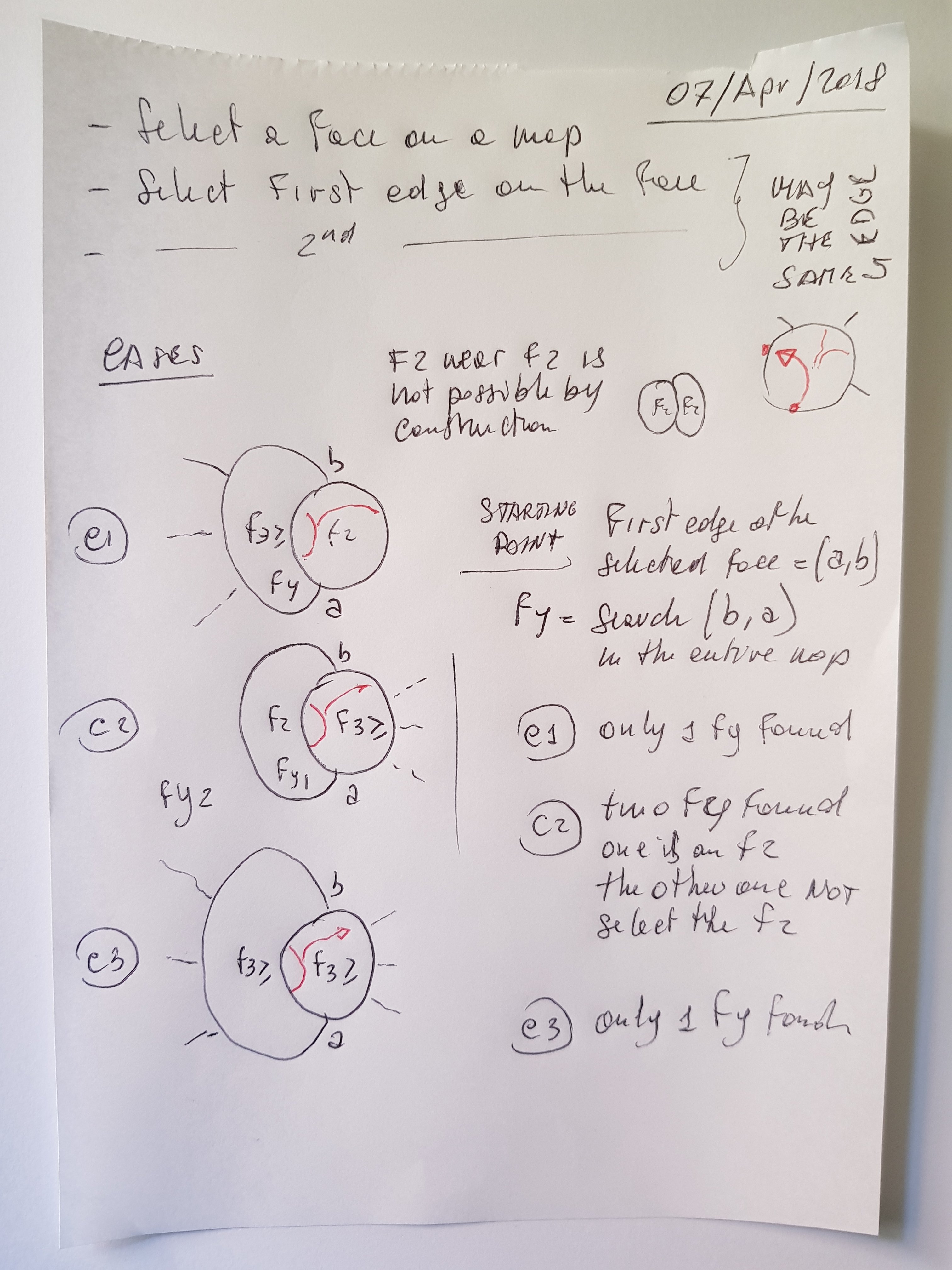
The other day, before going to sleep, I realized that I needed to revisit the problem, starting with a piece of evidence I had noticed long ago. When a map is colored, the corresponding Tait coloring of the borders creates color chains (R-G, R-B, or G-B) that always form loops. Moreover, there may be more than one loop for each pair of colors. For example, the map shown here has:
I wonder if analyzing how these loops form during the rebuilding phase of a map, after the reduction phase (see other posts), can lead me out of the mud.
Notes:
Once the map is completely four-colored (or 3-edge colored = Tait coloring), each chain (two-color chain) is actually a loop
This becomes clear when you consider the colors available at each vertex as you follow a chain. For example, if you’re examining the R-G chain and start from a vertex, following the Red color to the next vertex, that vertex will have the Green color available to continue the chain. As you keep alternating between R and G, each new vertex will offer the other color in the chain until you eventually return to the starting vertex, thereby closing the loop
If only one chain for a specific color selection (R-G, R-B, or G-B) exists, that chain touches all vertices of the map
If it weren’t so, one of the vertices not on the chain still would have the edges colored with three different colors, two of which (the same two colors of the chosen chain) would form another chain
The length of all loops is always an even number
This come straightforward from the definition of chain, multiple sequences of R and G = 2n
Deforming the original map, I managed to put in evidence the R-G loop, and then the other loops (R-B and G-B) respect to the first R-G deformation.
And here with the loops filled
Additional note:
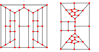
This was the map when I discovered that infinite random switches throughout the entire graph do not solve the impasse. It was bad 😦 The graph here is identical to the one in the previous post.
During the process of removing faces from a planar map (cubic planar graph) this video shows how the Euler’s equation redistribute its weights:
+4F2 +3F3 +2F4 +1F5 +0F6 -1F7 -2F8 -3F9 …. = 12
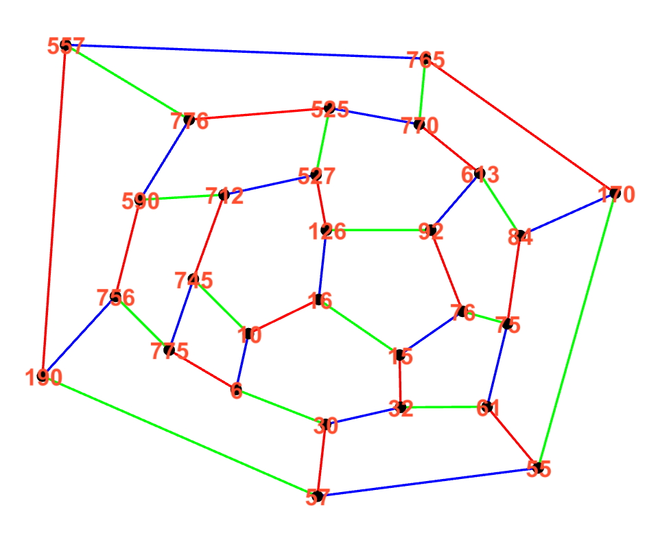
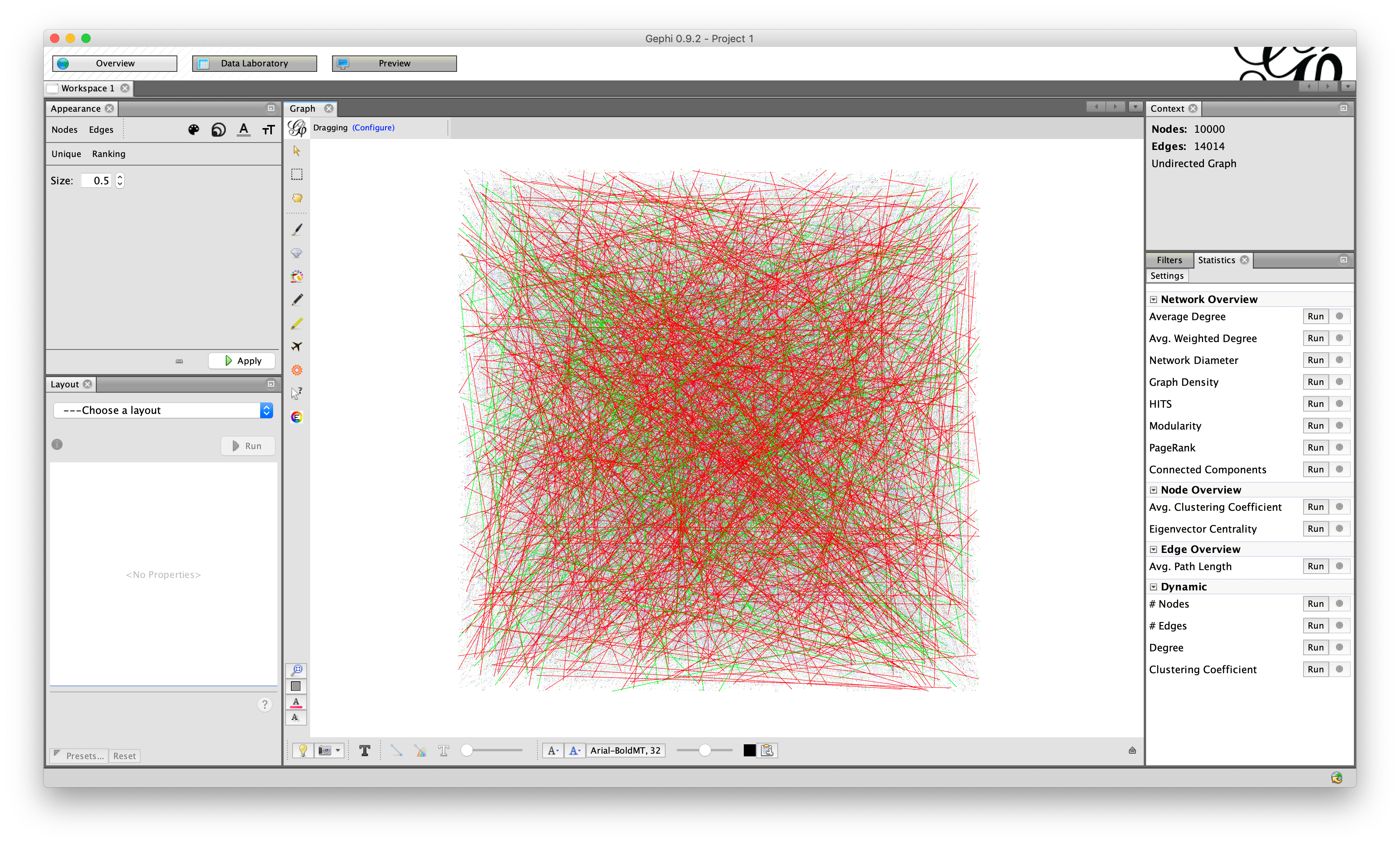
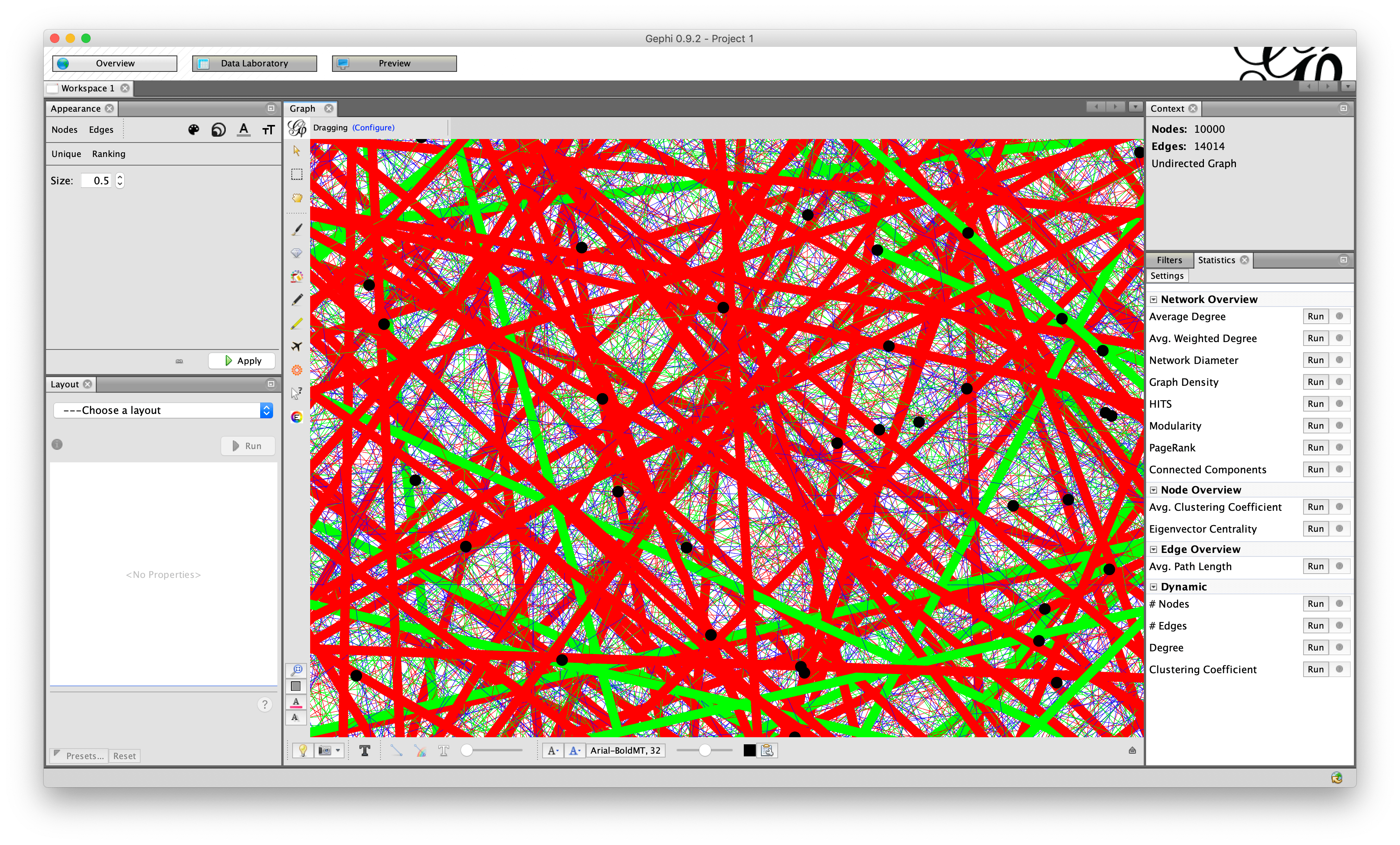
The map that has been used to produce this video is represented by a planar cubic graph made of almost 10000 faces (20000 vertices and 27972 edges).
The selection for the edges to remove that I used was: take an edge from an F2. Then, if no F2 exist, use an F3. And then, if no F3 exist, use an F4 and finally an F5.
A graph with 20000 vertices opened by Gephy appears as a black square 😦
Here is the .dot file and the planar representation of the map.
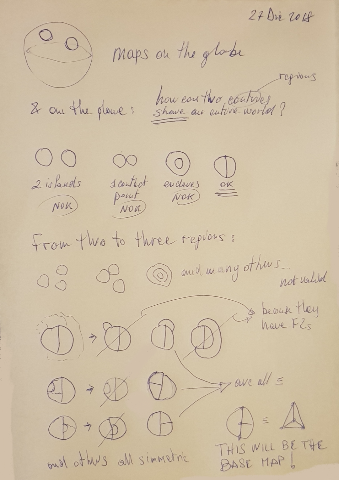
The four color theorem appeared in 1852, talking about the problem of coloring real maps. Let’s examine some basic aspects of these maps in relation to the four color theorem.
A world with just water and one land with no divisions, topologically equivalent to a disk, needs only two colors to paint the land and the ocean. This is the beginning, as the Pangea on Earth long ago.
If two parties want to share this land and both want to have access to the ocean and have contiguous regions, there is only one possible configuration, and the resulting map can be represented by a planar graph with 2 vertexes and 3 edges (multiedge graph). The other solutions that have been excluded by the two restrictions: “have access to the ocean” and “contiguous regions” are not so interesting for the scope of the theorem (see previous post).
If a third party comes into play, the initial region (surrounded by the ocean) has to be split among three parties, with the same two restrictions as stated before: “have access to the ocean” and “be contiguous regions”. If we consider all possible combinations, we can also see that among them there are some that can be eliminated introducing a third rule: “all faces have to touch each other”. This third rule can be added because all the configurations in which the three faces don’t touch each other contain F2 faces and therefore (is it to be proved?) can be eliminated. It will then rest only one configuration that meet all criteria, that is the one printed at the bottom right of the previous post image.
There are some methods around to create planar graphs. One of these is based on the Delaunay triangulation algorithm from which you can derive its dual, a 3 regular planar graph. Tools and libraries that I found around (sage, networkx and others), permits you to save the graph using one of common format to represent the graph itself, specifically: .dot, .graphml, .GEXF, .gpickle and others). One problem that I found is that if I save the graph I loose the planar representation of it.
Since for what I am trying to do, namely demonstrate with pencil and paper that the four color theorem has a simpler demonstration, I need to work directly with the planar representation of the graph.
I decided to implement my own method (based on edge addition to planar graphs. See “John M. Boyer and Wendy J. Myrvold, On the Cutting Edge: Simplified O(n) Planarity by Edge Addition. Journal of Graph Algorithms and Applications, Vol. 8, No. 3, pp. 241-273, 2004.”) to generate an save the graph directly using its planar representation. Get the code here at: https://github.com/stefanutti/maps-coloring-python. The program generates random planar graphs without using graphs library and most importantly without using complex algorithms, as planar embedding or planarity testing.
Planar embedding: “A combinatorial embedding of a graph is a clockwise ordering of the neighbors of each vertex. From this information one can define the faces of the embedding”.
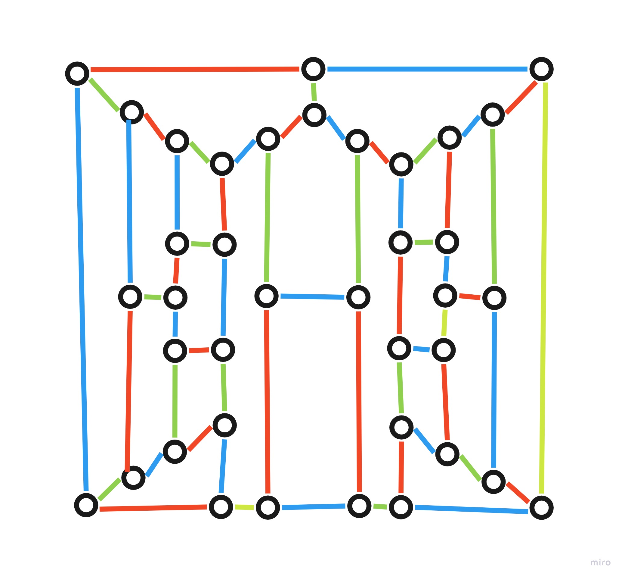
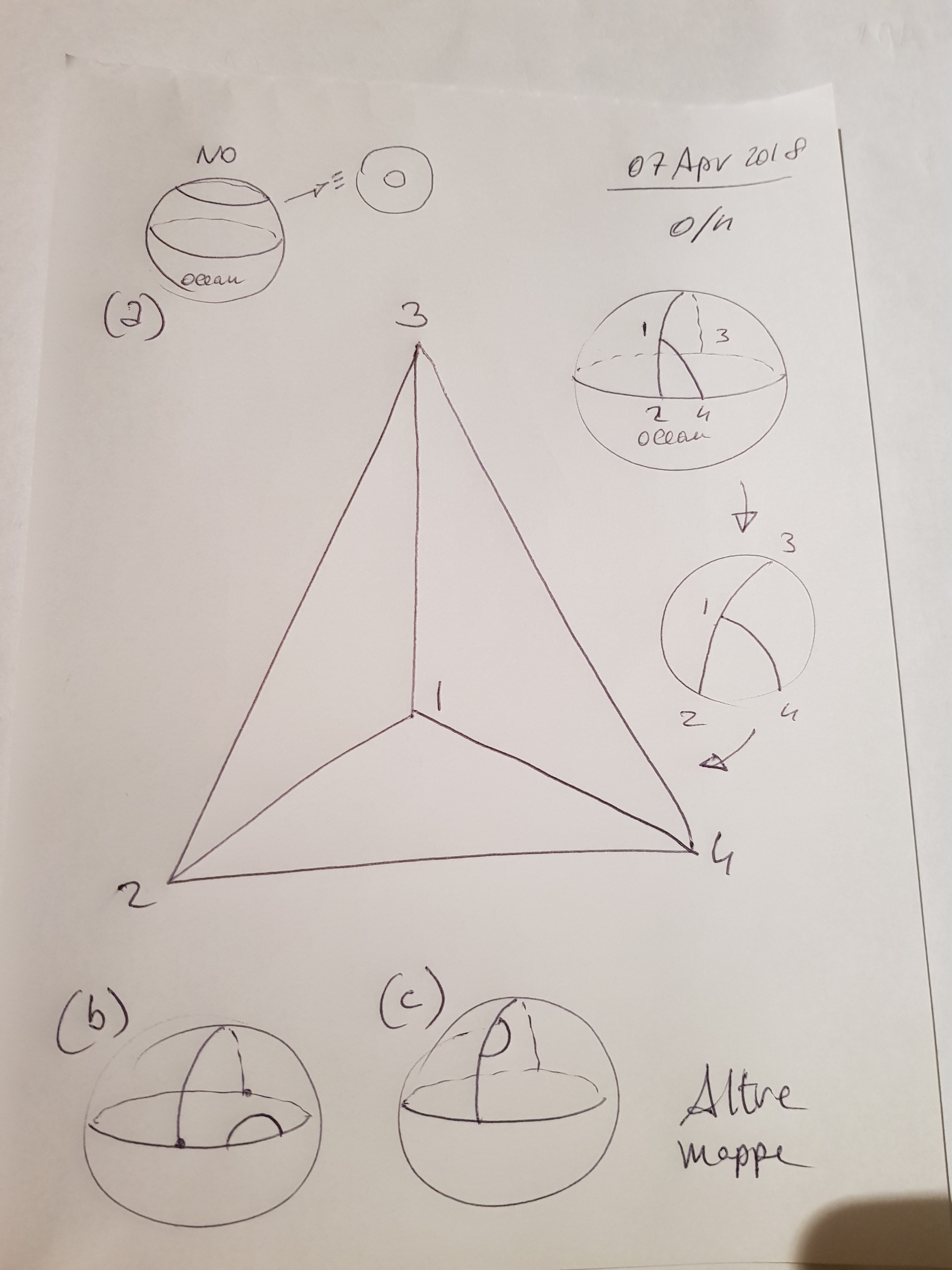
Edge addition can start from a basic graph of four faces (bottom right). In the third last line of this picture I added edges from a graph with 3 faces and 2 vertices (considering the ocean). But as you can deduct from the other pictures I can safely start from a graph with 4 faces and 4 vertices (bottom right).