Some questions about the previous post:
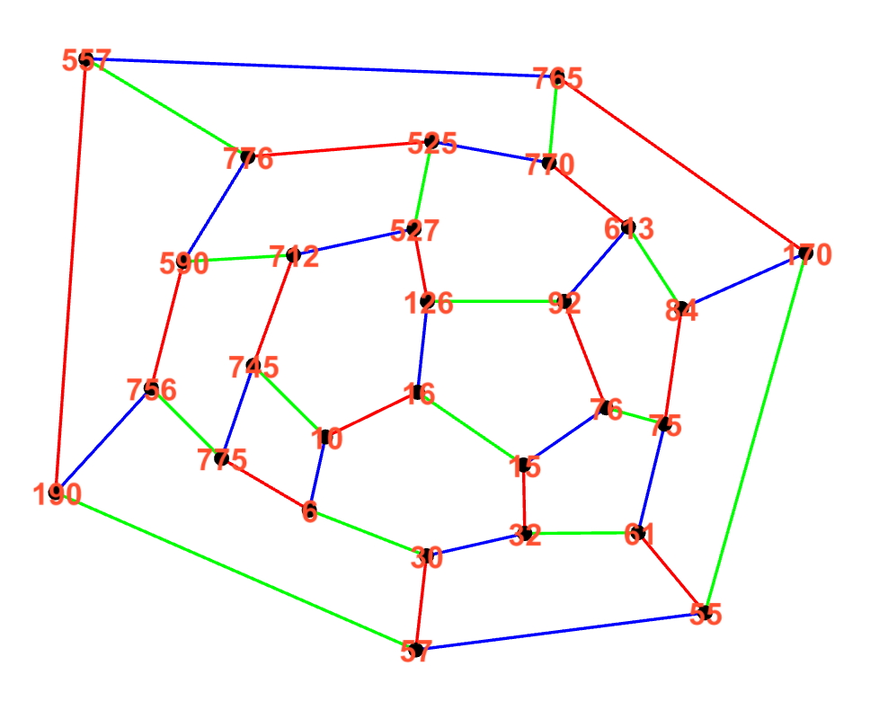
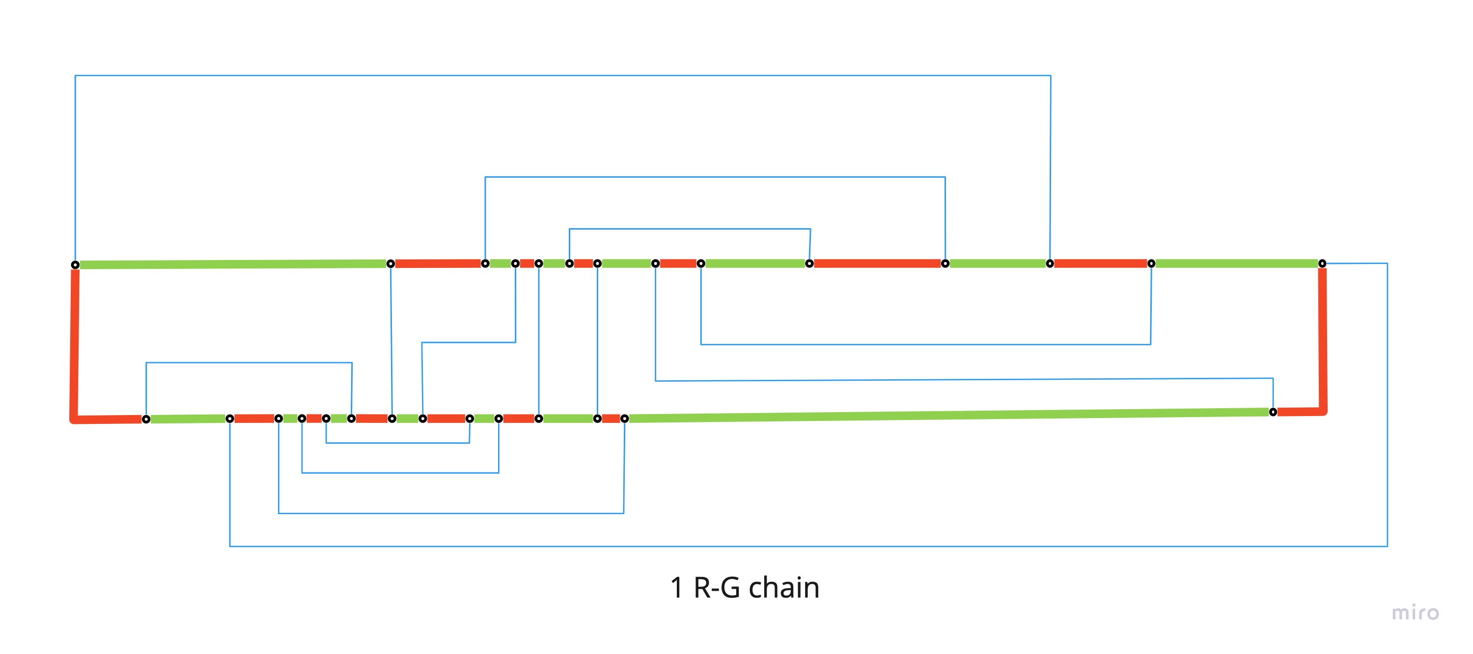
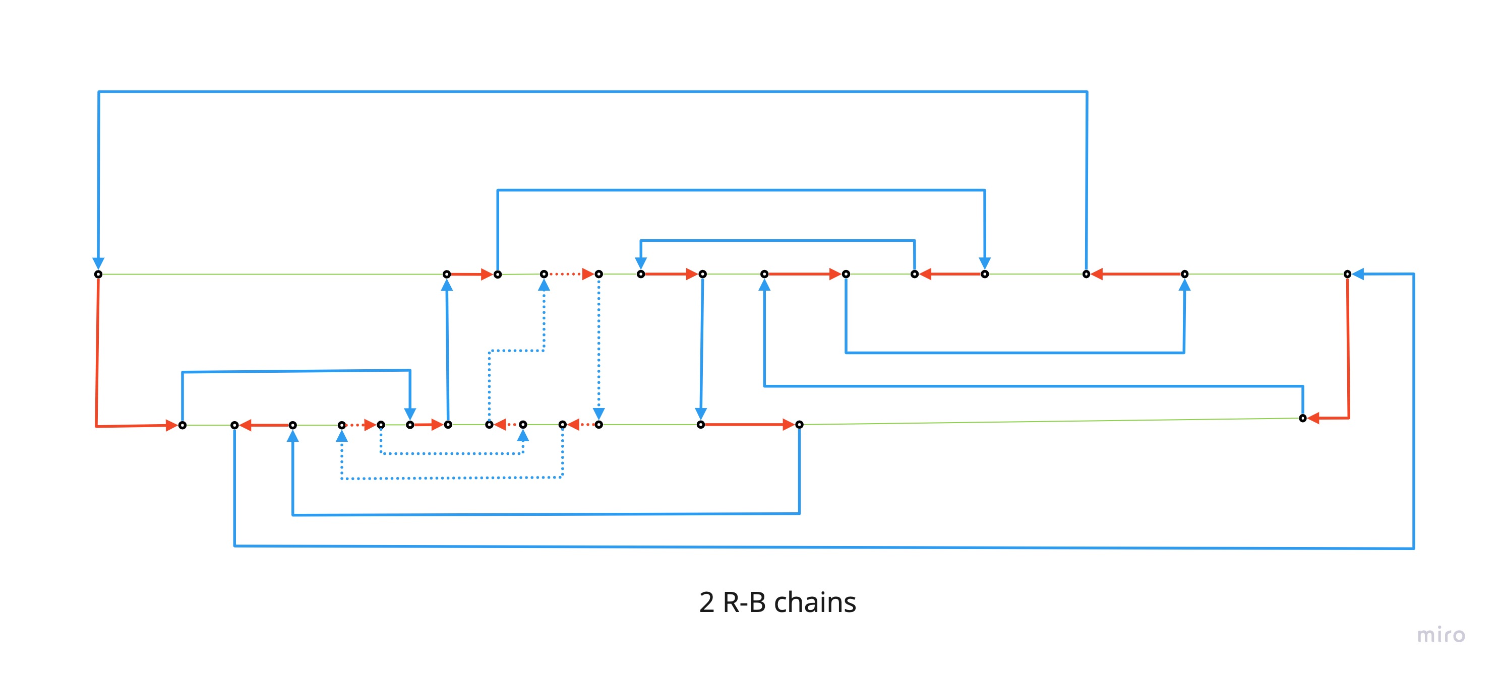
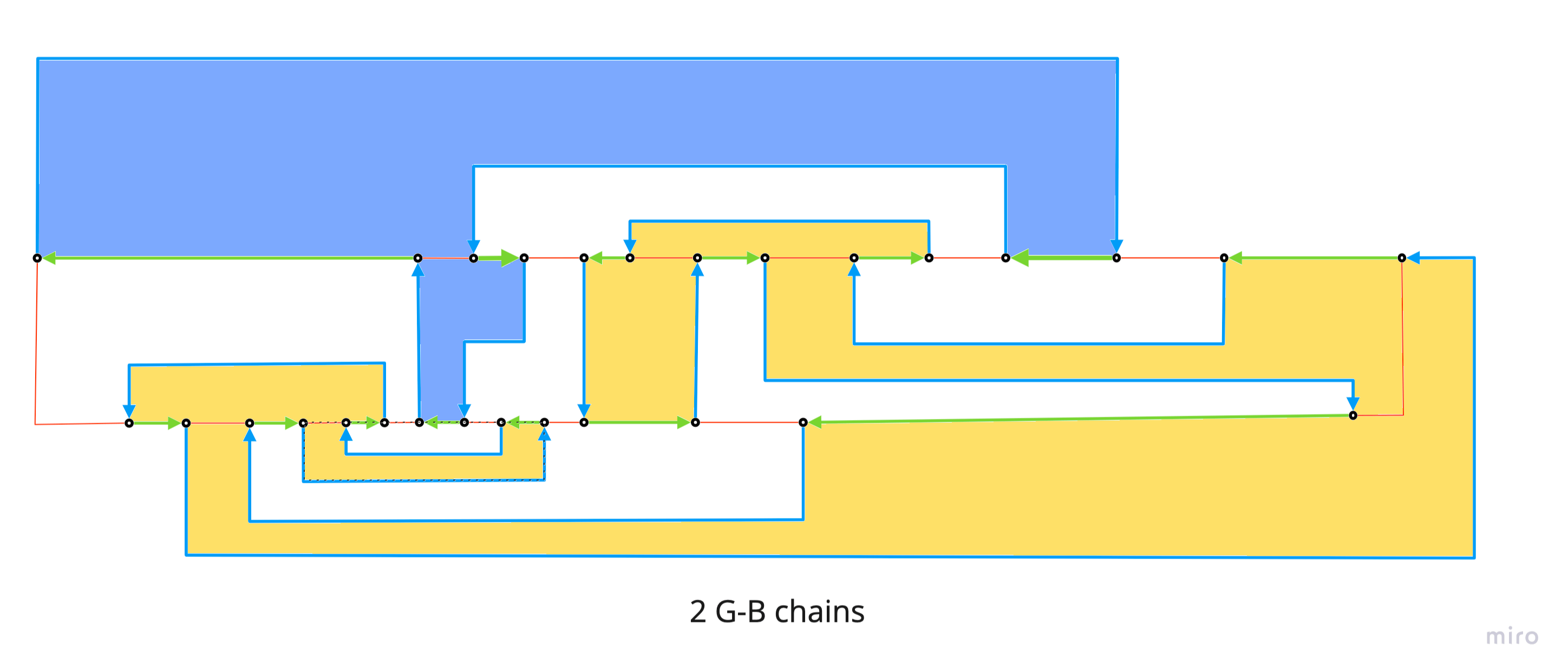
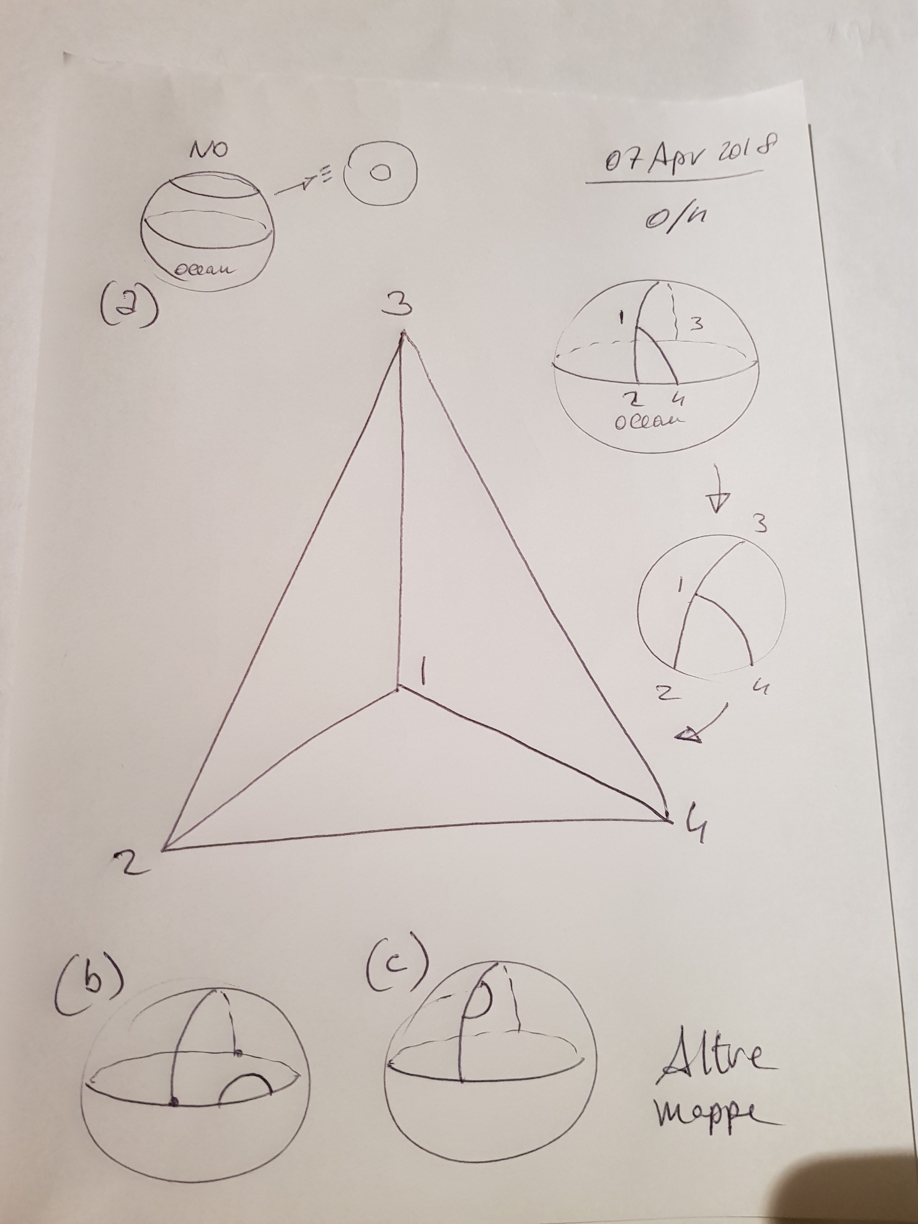
Q1) Can cycles be concentric?
Yes, see this example.
Q2) Verify if at least one of the cycles (R-G, R-B, or G-B) form an Hamiltonian circuit
False.
From the Tait’s conjecture we now know (now = 1946 by William Thomas Tutte) that 3-regular graphs exist also without an Hamiltonian circuit. It means that, no matter what, it is not possible to find a cycle that touches all vertices, and therefore no single Kempe cycles of any two color selection, can exist.
From Wikipedia, the free encyclopedia
This article is about graph theory. For the conjectures in knot theory, see Tait conjectures.
In mathematics, Tait’s conjecture states that “Every 3-connected planar cubic graph has a Hamiltonian cycle (along the edges) through all its vertices“. It was proposed by P. G. Tait (1884) and disproved by W. T. Tutte (1946), who constructed a counterexample with 25 faces, 69 edges and 46 vertices. Several smaller counterexamples, with 21 faces, 57 edges and 38 vertices, were later proved minimal by Holton & McKay (1988). The condition that the graph be 3-regular is necessary due to polyhedra such as the rhombic dodecahedron, which forms a bipartite graph with six degree-four vertices on one side and eight degree-three vertices on the other side; because any Hamiltonian cycle would have to alternate between the two sides of the bipartition, but they have unequal numbers of vertices, the rhombic dodecahedron is not Hamiltonian. The conjecture was significant, because if true, it would have implied the four color theorem: as Tait described, the four-color problem is equivalent to the problem of finding 3-edge-colorings of bridgeless cubic planar graphs. In a Hamiltonian cubic planar graph, such an edge coloring is easy to find: use two colors alternately on the cycle, and a third color for all remaining edges. Alternatively, a 4-coloring of the faces of a Hamiltonian cubic planar graph may be constructed directly, using two colors for the faces inside the cycle and two more colors for the faces outside.
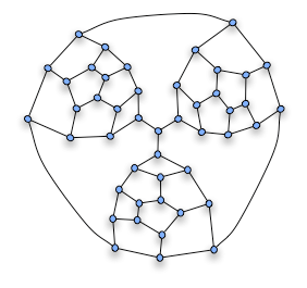
Smallest known non-Hamiltonian 3-regular planar graph: https://mathworld.wolfram.com/Barnette-Bosak-LederbergGraph.html.

Next post will be on the four coloring of the barnette-bosák-lederberg graph, which is the smallest known non-Hamiltonian graph, and the analysis of its Kempe cycles.
Q3) What about if I start with finding cycles, of even length (# of edges), that cross all vertices?
Some initial considerations: If cycles have to fit with Kempe cycles (closed paths of two alternating colors), they have to be of even length, and that would also mean that the total number of vertices crossed by all the cycles of the same two colors should be even too. Is it like this, or am I missing something? What about graphs with an odd number of vertices? Am I missing something?
Answer to the initial consideration: https://math.stackexchange.com/questions/181833/proving-that-the-number-of-vertices-of-odd-degree-in-any-graph-g-is-even + https://math.stackexchange.com/questions/181833/proving-that-the-number-of-vertices-of-odd-degree-in-any-graph-g-is-even
Finding cycles seems to be as difficult as finding a solution for of 4 coloring problem 😦